KiPI Tutorial
One real board taken through all three of KiPI's analyses, every click shown: a DC voltage drop and heating solve, an AC impedance solve, and a Coupled Noise solve. Each part starts from a new, empty setup.
About this tutorial
The User Guide describes every control in KiPI. This tutorial uses them in order on one board, the way you would on your own: what to enter, where the numbers come from (the schematic, a datasheet, a quick sum) and how to read what comes back. The Solver Guide explains what each solver does underneath.
The three parts stand alone, so you can go straight to the one you need:
| Part | Question | You enter |
|---|---|---|
| 1. DC | Does every part get the voltage it needs with all the loads drawing current, and how hot does the copper get? | VRMs, series links, loads, thermal limits |
| 2. AC | How low is the supply's impedance seen from a chip's power pins, from kHz to hundreds of MHz, and is it below the chip's target? | VRMs with their loop bandwidth, series links with ESL, capacitor models, probes and targets |
| 3. Coupled Noise | How much of a buck converter's switching noise reaches a nearby signal, and does it stay inside the receiver's noise margin? | The switcher (aggressor), the signal (victim), capacitor models |
Each part starts from a board with no setup, so each one lists everything that part needs, even where another part has entered it already. On your own board the three share one setup file: VRMs, series links and capacitor models entered once serve every mode.
The example board
The board is rev A of the Audio Visualiser DSP board: a dsPIC33AK digital signal processor that samples audio and drives two LED panels. It is an 8-layer, 1.574 mm board with 406 footprints. Its power tree:
+12Vin), through the
TPS259474 eFuse U201 and the 10 mΩ current-sense resistor R207 onto +12V.+12V. Together they are nearly all of the board's power.+12V,
through the 2.2 µH inductor L401 and the 20 mΩ sense resistor R406 onto
+3.3V. It remote-senses +3.3V through its feedback divider
R409/R410.+3.3VA_DSP (the dsPIC's analog supply, returned on GNDA_DSP
through FB702), R610 feeds the 8 MHz oscillator X601, and the Schottky diode D1001 feeds
a DS1683.+5V_USB; the CP2104 USB-UART bridge U901 makes
+3.3V_USB with its internal regulator.Every current, tolerance and part value used below comes from that board's schematic and its parts' datasheets.
Opening the board
- As a KiCad plugin: open the board in KiCad's PCB editor and click the KiPI toolbar button. KiPI refills the zones and reads the board from the editor (Starting KiPI).
- Standalone: start KiPI with its launcher, click Open… and pick
Audio_Visualiser_DSP.kicad_pcb. Standalone KiPI reads the zone fills saved in the file and cannot refill them, so fill the zones in KiCad (B) and save before opening.
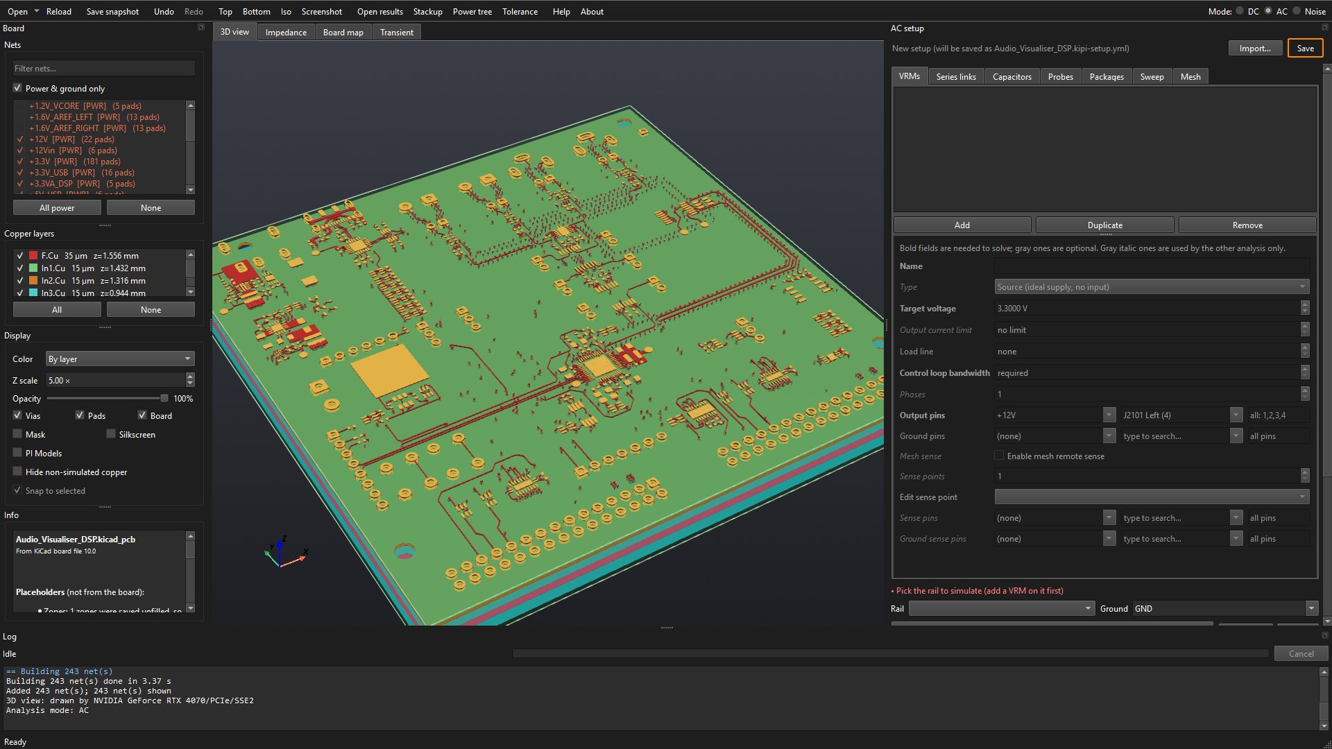
Either way, KiPI draws every net of the board in 3D. With no setup file beside the board, the PI setup panel on the right shows New setup (will be saved as Audio_Visualiser_DSP.kipi-setup.yml), and in red under its tabs, what it needs first: Add a VRM (the source of a net) to start.
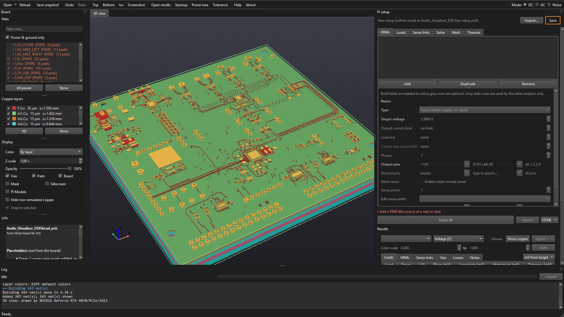
To start a part over from nothing on a board that already has a setup, rename or move
its .kipi-setup.yml and read the board again.
Part 1: DC voltage drop and heating
A DC solve puts every load's current through the copper at once and finds the voltage at every pin. It answers: does each part get a voltage inside its tolerance, which copper carries the current, and (with the electro-thermal solve) how hot does it get? You tell KiPI where the power comes from (VRMs), what passes it from one net to the next (series links) and what draws it (loads).
Tick the nets to analyze
The Nets list on the left decides which copper is solved and which nets the setup's pin pickers offer. With Power & ground only ticked it lists the nets that look like power or ground (by name, net class and zones), and KiPI ticks a first guess.
Tick every net that current flows through, from each source to each load and back:
| Nets | Why |
|---|---|
+12Vin, Net-(U201-OUT), +12V |
The input: J201 → eFuse U201 → R207 → the 12 V plane. The eFuse's output has no name
in the schematic, so KiCad calls it Net-(U201-OUT). Untick
Power & ground only or type in the filter box to find nets like it. |
Net-(C406-Pad1), +3.3V | The buck's output (L401 to R406) and the 3.3 V rail. |
+3.3VA_DSP, Net-(X601-Vdd),
Net-(D1001-K) | Behind FB701, R610 and D1001. A net a series link joins to a rail is solved with it even unticked, but tick it anyway: the AC mode's Capacitors table lists only capacitors on ticked nets (Part 2 shows what happens otherwise). |
+5V_USB, Net-(FB901-Pad2), Net-(U904-EN),
+3.3V_USB | The USB side. |
GND, GNDA_DSP | The returns. |
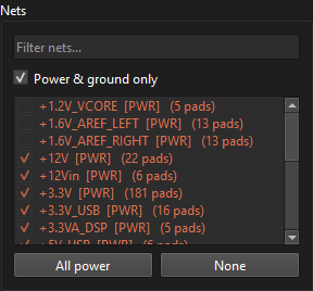
Leave out nets nothing flows through for this analysis (the analog references
+1.6V_AREF_*, for example): every ticked net is meshed, and a net with no source
is reported as not driven.
Add the VRMs
A VRM is anything that holds a net at a voltage: a connector from a bench supply, a regulator, a battery. Open the VRMs tab and click Add.
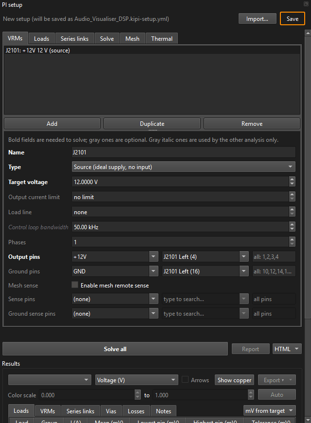
+12V), 12 V read from the net's name, and the part's ground
pins.KiPI's guess is a start, not the answer. The 12 V really enters at the barrel jack J201,
on +12Vin. Change it with the pin picker:
the first box is the net, the second the part (type to search: j201), the third
optional pin numbers (blank means every pin of that part on that net).
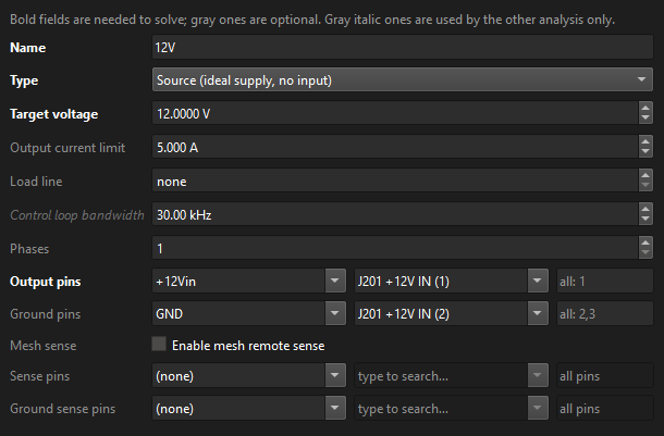
The 12 V input: a source
| Field | Value | Where it comes from |
|---|---|---|
| Name | 12V | Any name; it labels the results. |
| Type | Source | An ideal supply with nothing upstream on the board. |
| Target voltage | 12 V | The adapter's voltage. |
| Output current limit | 5 A | Optional. What the input may supply; the VRMs table gives PASS or FAIL against it. |
| Output pins | +12Vin · J201 | Where the current enters the copper. |
| Ground pins | GND · J201 | Optional, but with them the ground return is solved too, and every load is judged on its supply minus its ground. |
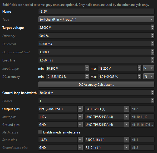
The 3.3 V buck: a switcher with remote sense
Click Add again for U402. For a switcher, Output pins are where it drives
the rail. Here that is the inductor's output side, L401 on Net-(C406-Pad1),
since the copper from U402 to L401 carries switched current, not the DC output. Picking the
output part fills Input pins (U402 on +12V) and Ground pins.
| Field | Value | Where it comes from |
|---|---|---|
| Type | Switcher | Pin = Pout / η:
its input current on +12V follows from what it delivers. |
| Target voltage | 3.3 V | The rail's nominal; loads are judged against it. |
| Efficiency | 90 % | Read off the TPS62150A's efficiency curve for 12 V in, 3.3 V out at this load. |
| Output current limit | 1 A | The TPS62150A is a 1 A part. |
| Load line | 1.65 mΩ | Optional droop with load: here it stands for the converter's load regulation. |
| Input range | 10.8 to 13.2 V | 12 V ± 10 %, the input the design must hold regulation over. |
| DC accuracy | −2.16 % / +4.04 % | The output's DC error: the reference's accuracy and the R409/R410 divider tolerances, which DC Accuracy Calculator… adds up. The AC target calculator uses it. |
| Control loop bandwidth | 50 kHz | Used by AC only (Part 2). |
| Sense pins | +3.3V · R409 | The top of the feedback divider connects to the rail at R409's pad, after R406, so the buck regulates 3.3 V there, not at its own pins. |
| Ground sense pins | GND · R410 | The divider's bottom resistor: the ground the feedback is measured from. |
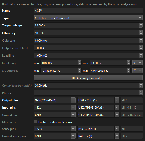
+12V, remote sense at
the feedback divider.The USB side: a source and an LDO
+5V_USB is a Source of 5 V on J901's VBUS pins
(Net-(FB901-Pad2)). +3.3V_USB is the CP2104's internal regulator: an
LDO on U901, output +3.3V_USB, input +5V_USB. From the
CP2104 datasheet's regulator figures: 3.45 V out, 0.12 mA quiescent, 100 mA for other parts, a 3.0 to
5.25 V input, and an output between 3.3 and 3.6 V (entered as the DC accuracy, in
V).
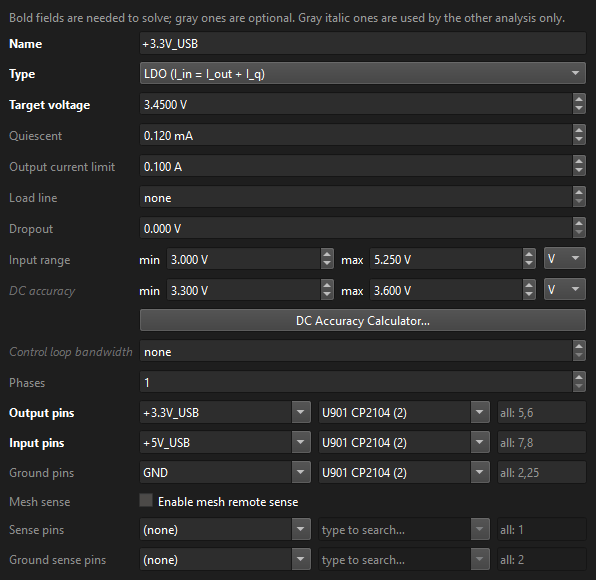
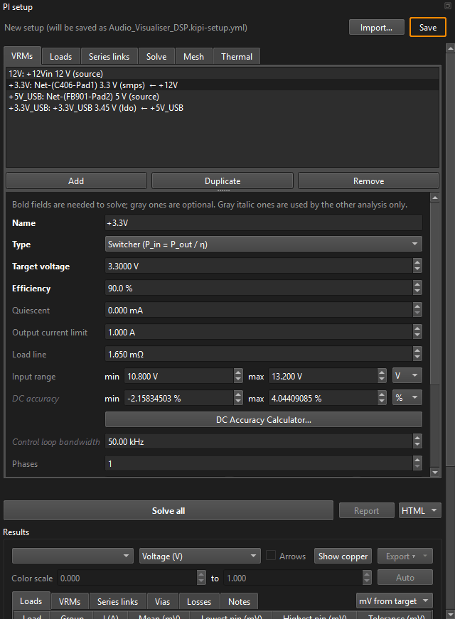
← +12V).Add the series links
A series link is a part that passes DC from one net to another: a sense
resistor, a ferrite bead, a fuse, a load switch, a diode. Without them,
Net-(U201-OUT) is a net nothing drives and the 12 V never reaches
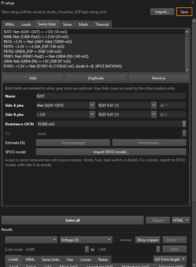
+12V; the red list under the tabs says so. Open Series links and
Add one per part. Pick Side A; for a two-terminal part KiPI fills in
Side B on its other net, and for a resistor reads the Resistance from its value.
| Link | Between | Resistance | Where it comes from |
|---|---|---|---|
| U201 | +12Vin → Net-(U201-OUT) | 28.2 mΩ | TPS259474 eFuse: its on-resistance from the datasheet. An IC that passes current from pin to pin is a series link too. |
| R207 | Net-(U201-OUT) → +12V | 10 mΩ | Read from its value, 0.01. |
| R406 | Net-(C406-Pad1) → +3.3V | 20 mΩ | Read from its value. |
| R610 | +3.3V → Net-(X601-Vdd) | 10 Ω | The oscillator's supply filter resistor. |
| FB701 | +3.3V → +3.3VA_DSP | 140 mΩ | The ferrite bead's DCR (datasheet). Its ESL matters only for AC (Part 2). |
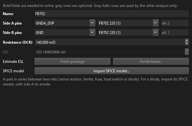
| FB702 | GNDA_DSP → GND | 140 mΩ | A link between two grounds: the analog ground's ferrite. KiPI solves both grounds as one return. |
| FB901, U904 | VBUS → +5V_USB | 140, 97 mΩ | The USB ferrite and the TPD3S014's switch resistance. |
| D1001 | +3.3V → Net-(D1001-K) | (model) | A BAT43WS Schottky: imported from its SPICE model (below). |
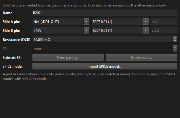
A diode from its SPICE model
A diode's drop changes with its current, so it is not a fixed resistance. Select the D1001
link with Side A on the anode (pin 2, on +3.3V) and Side B on the
cathode (pin 1), then click Import SPICE model… and pick the maker's model file.
For the BAT43WS that is Taiwan Semiconductor's BAT43WS.lib, which holds a
.MODEL BAT43WS D card. The dialog lists the file's diode models and two-pin
subcircuits and shows the forward voltage the model gives at 1 mA, 100 mA and 1 A.
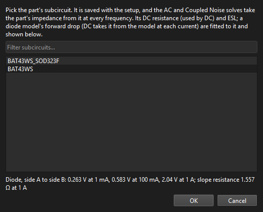
BAT43WS_SOD323F wrapper has
its pins in cathode, anode order, so the bare model, anode first, is the one to use with
side A on the anode.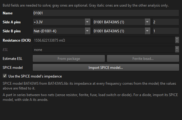
Add the loads
A load is a part that draws current from a rail: give its supply pins, its current and, to get a PASS or FAIL, its tolerance. Picking the supply part fills its ground pins. Currents come from datasheets (the maximum supply current, or a calculated one for the firmware's use case); tolerances from each part's recommended operating supply range.
A connector load
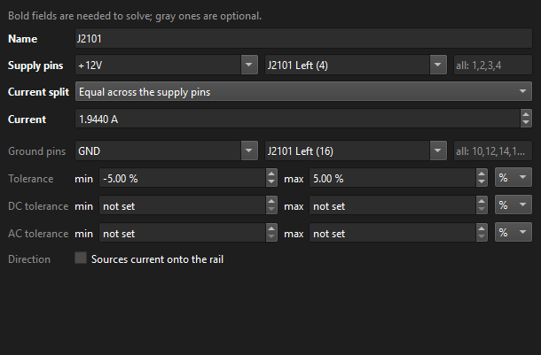
J2101 feeds an LED panel: 1.944 A from +12V, returned on GND. The panel
needs its 12 V within ±5 %. Enter Tolerance min −5 %, max +5 %.
A chip's power pins, and a tolerance in volts
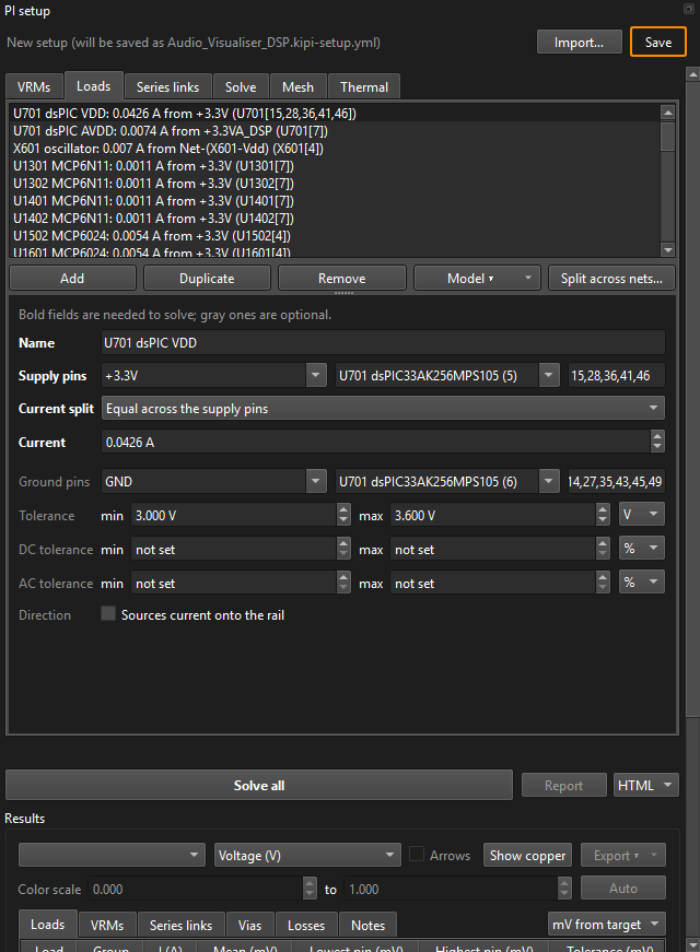
The dsPIC's digital supply: Supply pins +3.3V · U701, and pins
15,28,36,41,46 typed in the third box, since U701 has other pins on
+3.3V-connected nets. 42.6 mA, its supply current from the datasheet. Its datasheet gives the supply as 3.0 to 3.6 V, so set the unit box to V and
enter 3.0 and 3.6 directly.
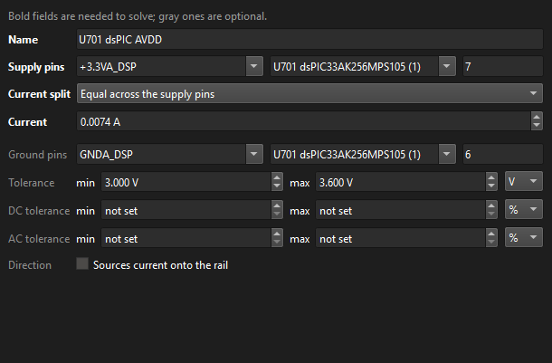
Its analog supply is a load of its own: +3.3VA_DSP · U701 pin 7, 7.4 mA,
ground pins on GNDA_DSP.
Different currents on different pins
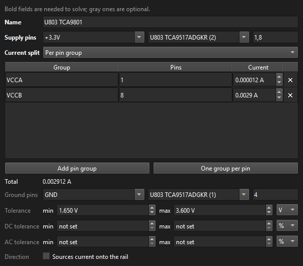
U803 (an I²C buffer) has two supplies on +3.3V, VCCA (pin 1) and
VCCB (pin 8), drawing very different currents. Set Current split to Per pin
group and add a row for each. The results' Notes list each group's voltage.
The rest
The same steps for every other part: the op-amps, logic, the encoder module, the status
LEDs (each LED's current, entered on its resistor's supply pin, with no tolerance, so it
gets no verdict) and the parts on +3.3V_USB. Parts fitted only sometimes are
still entered, with (DNP) in their names, so the setup is the worst case. This board
has 63 loads.
Check the power tree
Click Power tree on the toolbar. It draws the setup as a block diagram, left to right in the direction power flows: sources, regulators, rails, series links and loads. It is the quickest way to spot a link in the wrong place or a load on the wrong rail.
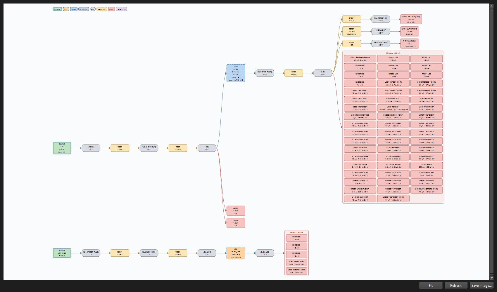
+12V, feeding J2101, J2102 and the
buck; the buck → R406 → +3.3V and its loads (packed in a grid), with FB701, R610 and
D1001 branching off; the USB chain along the bottom. Hover a block for its pins; Ctrl +
wheel zooms.Check the Solve, Mesh and Thermal tabs
The Solve tab lists the net groups KiPI will solve: each rail with every net a series link joins to it, and the grounds. Untick a group that is not routed yet to solve the rest. Here all five stay ticked.
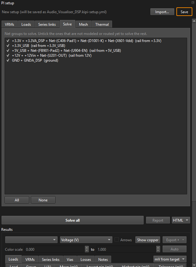
+3.3V takes in the four nets behind R406, FB701,
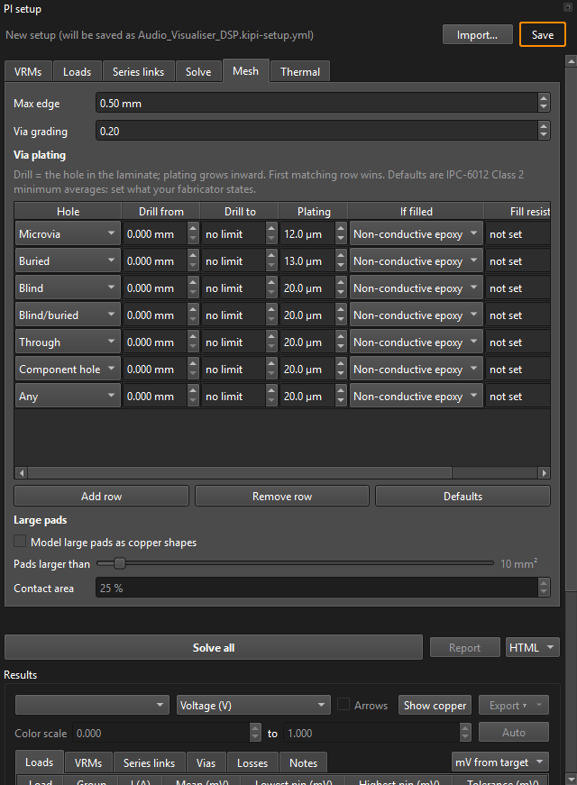
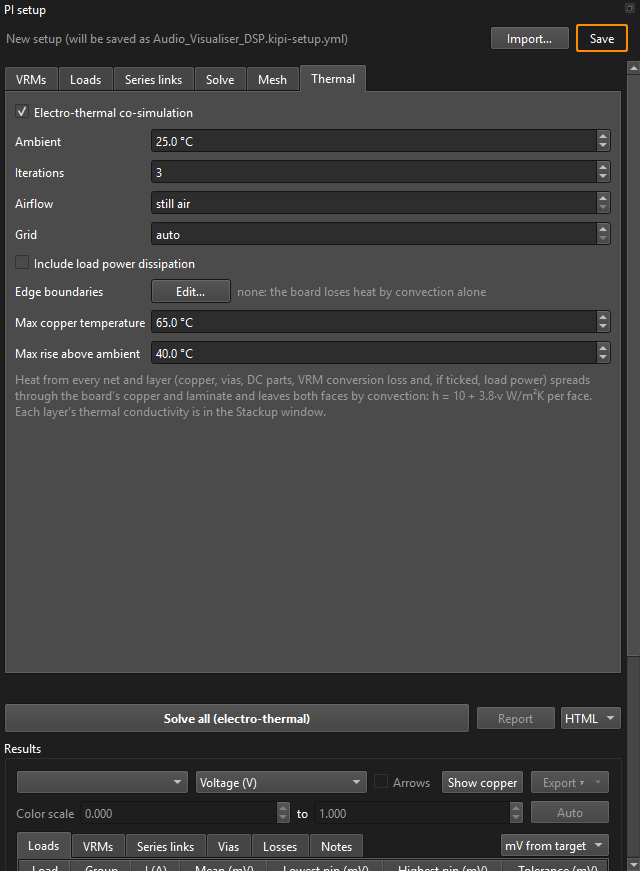
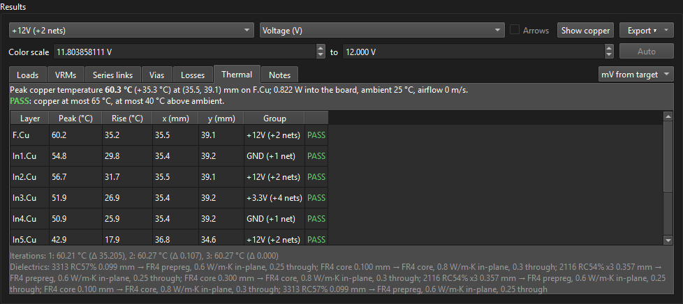
R610 and D1001; GND takes in GNDA_DSP through FB702.The Mesh tab's defaults suit most boards; set the via plating your fabricator states (here 25 µm). Then open Thermal and tick Electro-thermal co-simulation: the copper's losses heat the board and warmer copper resists more. Set the limits to judge it against: Max copper temperature 65 °C and Max rise above ambient 40 °C, at 25 °C ambient in still air.
Solve
The red list under the tabs is now empty. Click Solve all (electro-thermal). KiPI saves the setup next to the board, meshes the five groups and solves them, then heats the board with their losses and solves again, three times. The log shows each stage; this board took about a minute and a half. The biggest group is the ground: 2.1 million unknowns, as it fills three of the inner layers.
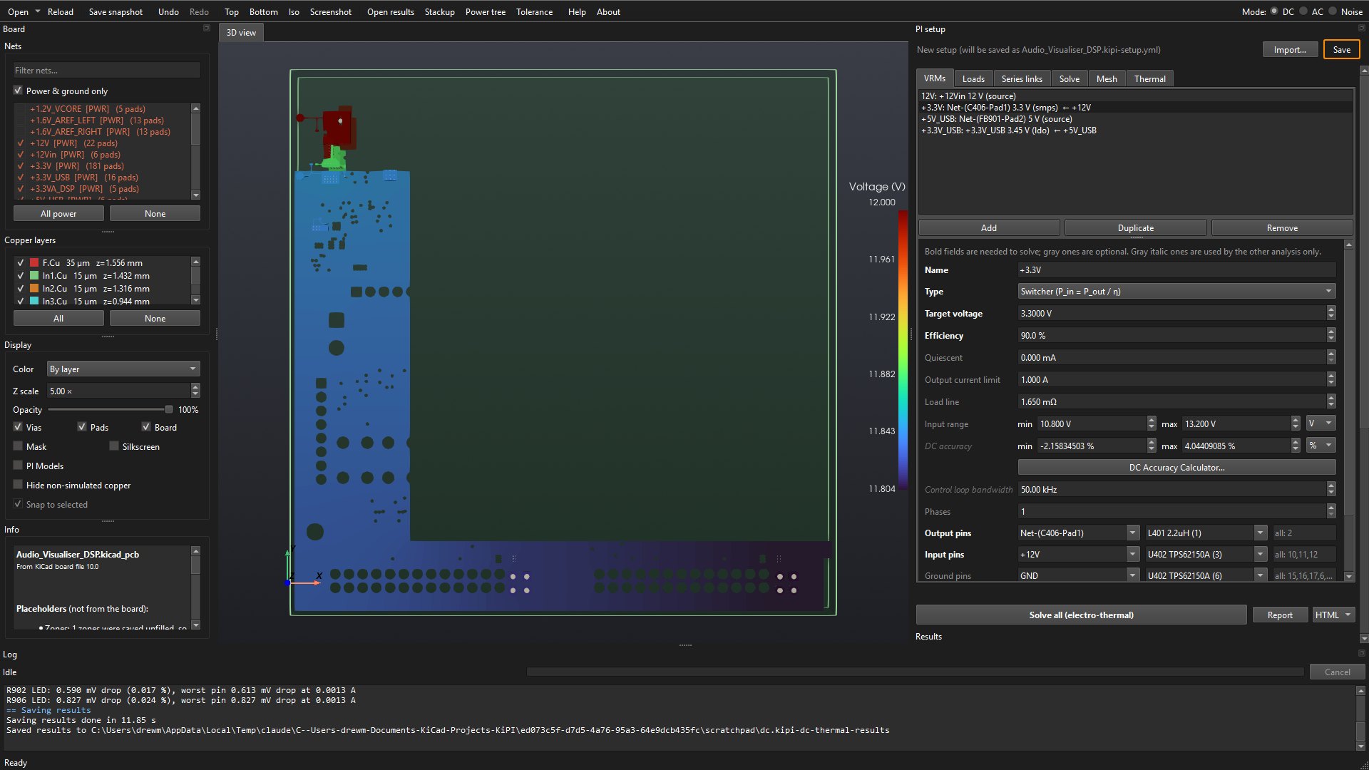
+12V group's voltage in 3D, the results
under the setup.Read the results tables
The Loads table gives each load's voltage, in mV from its VRM's target by default (the list at the right switches to % or volts), its lowest and highest pins, its tolerance, the margin left (negative and red when outside) and the verdict.
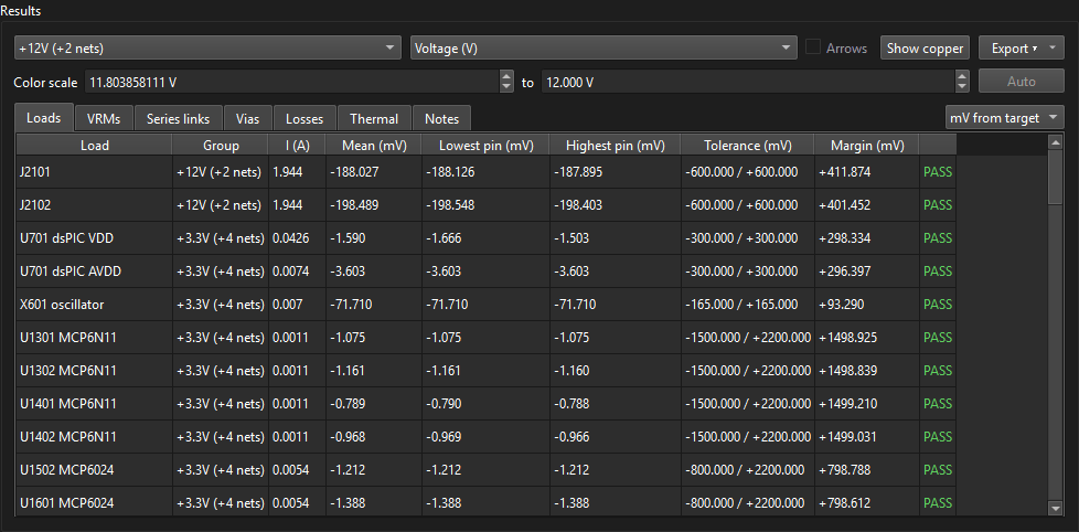
What the numbers say about this board:
- The LED panels lose 188 and 198 mV, about 1.6 % of 12 V. They draw 3.9 A between them, through the eFuse (28.2 mΩ: 110 mV), R207 (10 mΩ: 39 mV) and the copper.
- The dsPIC is within 2 mV of 3.3 V: the buck senses
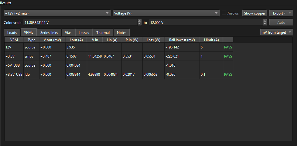
+3.3Vbeside it, and it draws little. - The VRMs table: the 12 V input supplies 3.935 A of its 5 A limit; the buck
delivers 151 mA and draws 47 mA from
+12V, which reaches it at 11.84 V, inside its 10.8 to 13.2 V input range.
Net-(D1001-K), beyond the diode.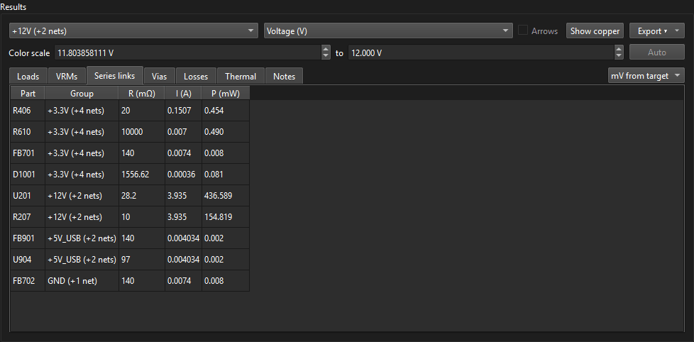
The Thermal tab gives the hottest copper on each layer:
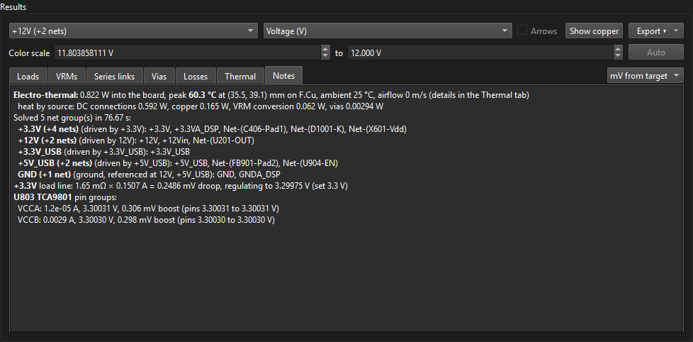
The Notes tab lists what was solved: each group's nets, the solve time, the buck's load-line droop, U803's pin groups and any warnings or parts left out.
Read the 3D view
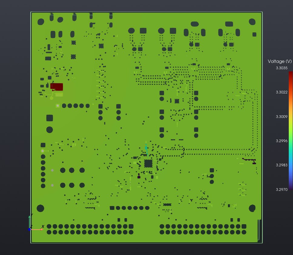
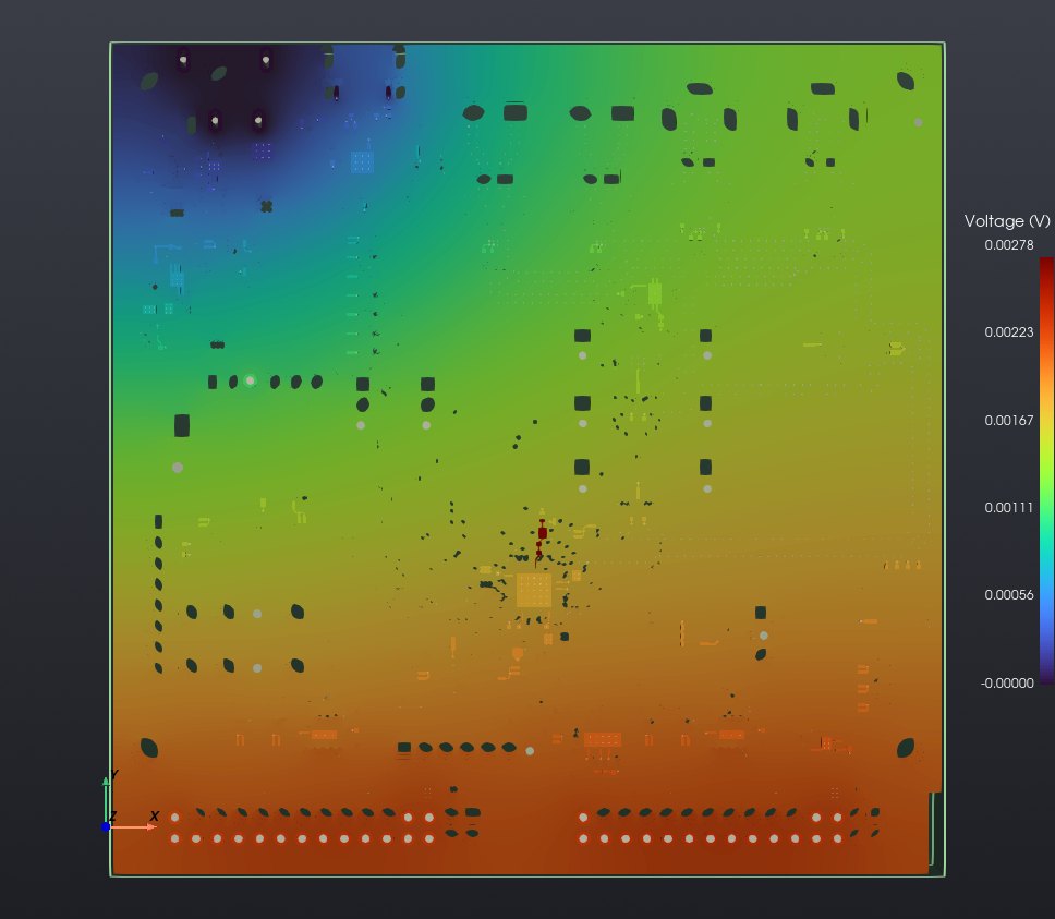
Pick a net group and a field above the tables to colour the copper. Click anywhere on the copper to probe: the Info box shows the exact value there. Top, Bottom and Iso on the toolbar set the camera.
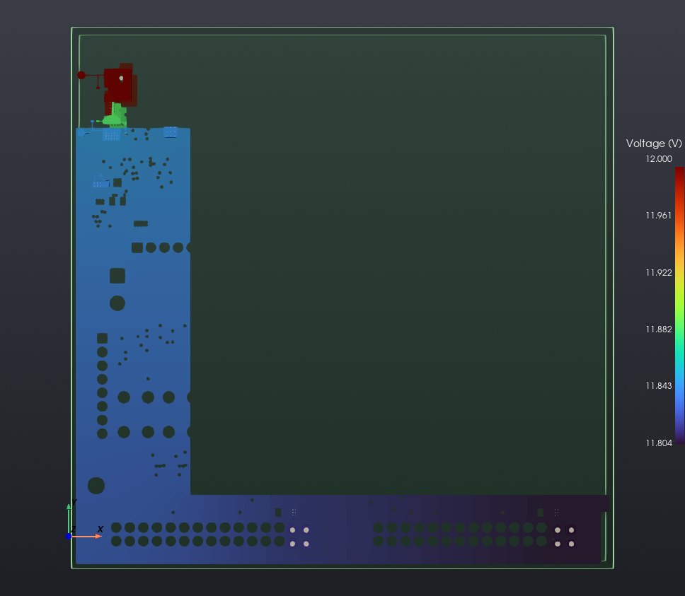
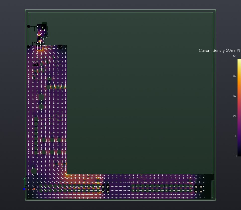
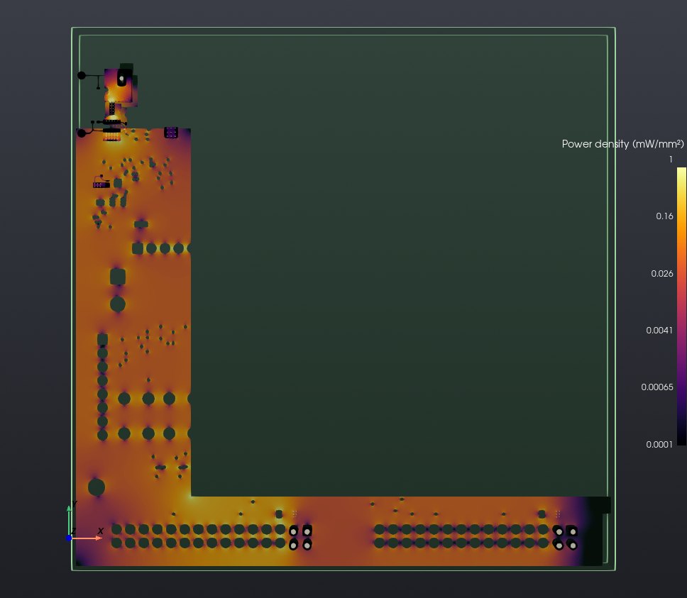
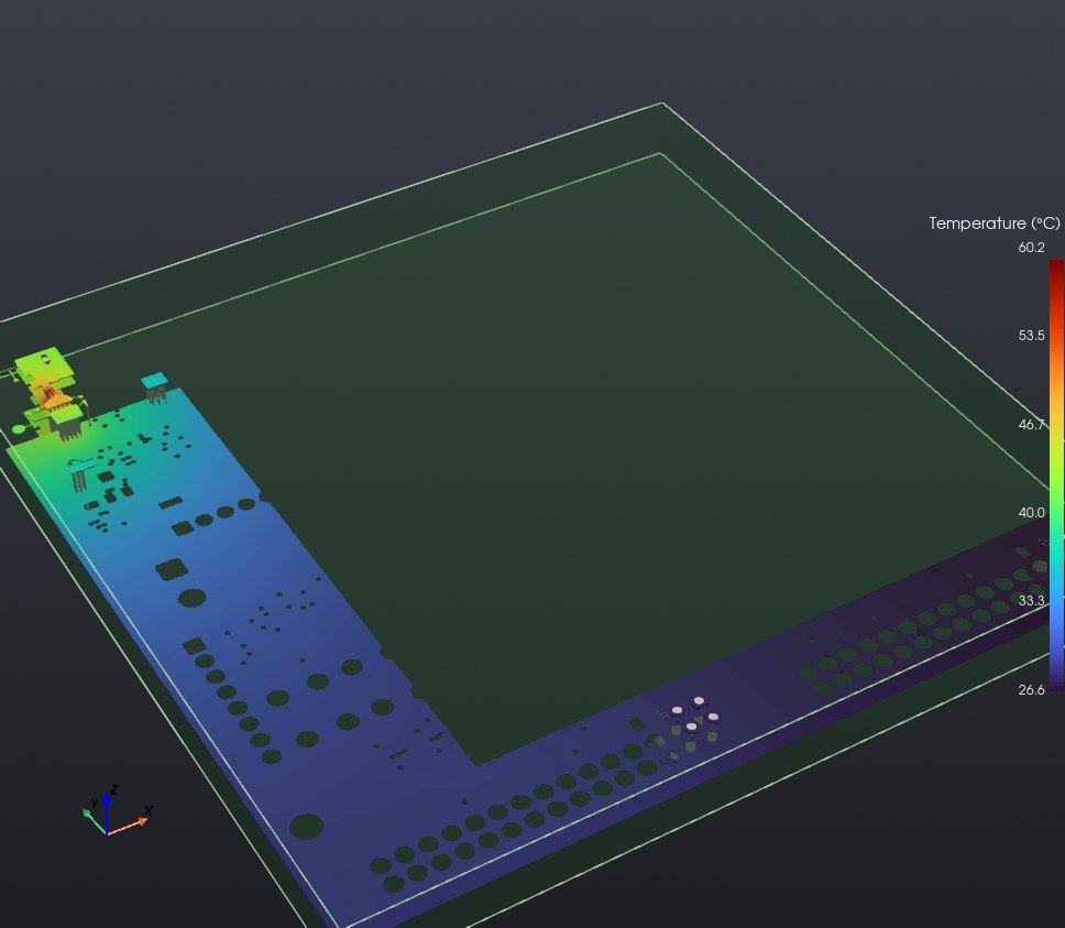
A rail with very little drop looks one colour on the whole-range scale. Type limits into Color scale to stretch the colours over the range you care about:
Report and save
- Report beside the Solve button writes a single-file HTML report next to the board (or a PDF, chosen beside it): every table, an interactive 3D view of each group, per-layer maps and the temperature map (details).
- Export ▾ → Save results… saves the solve, to open again with Open results… without solving.
- The setup was saved with the solve as
Audio_Visualiser_DSP.kipi-setup.yml; the next session starts from it.
When a result fails: the margin says by how much, the 3D current density shows where the copper is thin, and the Losses tab shows where the power goes. Change the layout in KiCad, then Load from KiCad (or Reload) and solve again; the setup stays.
Part 2: PDN impedance (AC)
A chip's current is not steady: it changes with every clock edge and every burst of work. The supply network (planes, vias and decoupling capacitors) has an impedance Z that varies with frequency, and a current change ΔI moves the supply by about ΔI·|Z|. The AC solve finds |Z| looking into a chip's power pins, from 1 kHz to 300 MHz here, and compares it with a target impedance: the most it may be for the supply to stay inside its AC tolerance.
This part starts from a new setup again. For an AC solve, KiPI needs the VRMs (they define each rail and its loop bandwidth), the series links (with their inductance), a model for each capacitor, and probes with their targets. Loads are not needed.
Switch to AC and tick the nets
Click AC beside Mode at the right end of the toolbar (or press Ctrl+2). The setup panel becomes the AC setup, with its own tabs. Tick the same nets as in Part 1: each rail, its ground, and every net a capacitor or series link on it connects to.
Add the VRMs, with their loop bandwidth
Add the VRMs as in Part 1: the same fields, the same pins. One field matters only here, and an AC solve cannot run without it: the Control loop bandwidth.
KiPI leaves the regulator out of the AC circuit, so the curve it draws is the open-loop impedance of the copper and capacitors, which keeps rising toward low frequency. Below its loop bandwidth (its gain crossover) the regulator holds the rail itself, so a target only applies above it. Find it in the regulator's datasheet or design tool, or measure it with a loop analyzer. A buck like the TPS62150A crosses over at tens of kHz: 50 kHz here. The 12 V adapter's response is slower: 30 kHz.
Add the series links, with their ESL
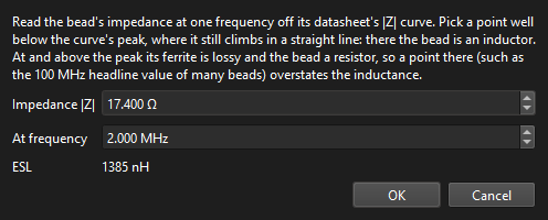
Add the same series links as in Part 1. In AC each link is its resistance plus its ESL (inductance), and a ferrite bead's inductance is what makes it a filter. For a chip resistor Estimate ESL → From package works it out from the footprint (0.4 nH for an 0402). For a bead, use Ferrite bead… and its datasheet's impedance curve.
FB701 (and FB702 and FB901) is a Murata BLM15EX221SN1D: 220 Ω at 100 MHz, 140 mΩ DCR. Murata's product page plots its |Z|, R and X against frequency. Read |Z| low on the curve, where R is still small and the bead is an inductor: 17.4 Ω at 2 MHz, with R only 1.7 Ω there. Not the 100 MHz headline: there R is 203 of its 229 Ω, and the bead is mostly a resistor. Even at 10 MHz (|Z| 78 Ω, R 32 Ω) the resistance would push the figure up.
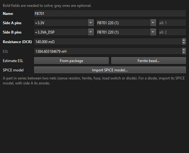
A bead's maker usually also gives a SPICE model of it. Import SPICE model… takes its impedance at every frequency instead, so the bead keeps its resistive peak.
Make the capacitor models
Every capacitor between a rail and its ground needs a model: its capacitance, ESL and ESR, shared by all the identical parts that use it. Open Capacitors and click Models from values: KiPI makes one model per distinct value among the capacitors on the ticked nets, with the capacitance read from the value.
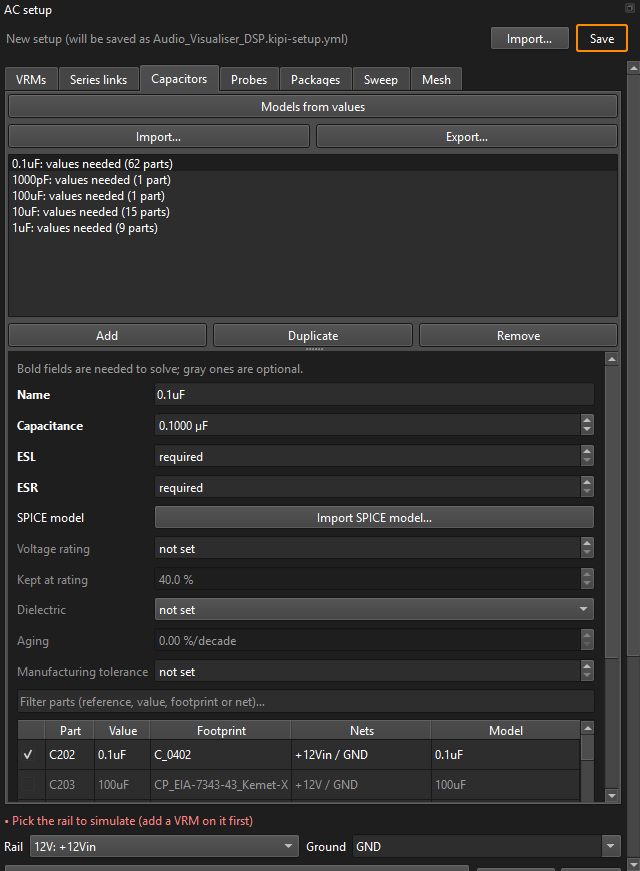
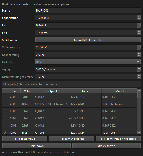
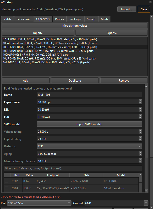
One model per value is too coarse here: this board's 10 µF parts are three different parts, an 0402, an 0805 and a 1206, each with its own ESL and DC bias. Make one model per part (Add, or Duplicate and rename), then select a row in the parts table and click Tick same value + footprint to give the model every part with that value and footprint. A part ticked here leaves its old model.
Read a capacitor's datasheet
Take C402 and C403, the buck's 12 V input capacitors. Their Digi-Key PN field gives 445-6862-1-ND, a TDK C3216X5R1E106K160AB: 10 µF ±10 %, 25 V, X5R, 1206. TDK's product page for it gives the ratings in a table and the rest in its Characteristic Graph section: impedance, ESR, capacitance and DC bias curves, each readable value by value by hovering over the curve.
| KiPI field | Value | Where on the datasheet |
|---|---|---|
| Capacitance | 10 µF | The nominal value, at 0 V and 25 °C. KiPI derates it for DC bias itself (below). |
| ESL | 0.82 nH | From the Impedance graph, on its rising (inductive) side well above resonance, where |Z| ≈ 2πf·ESL. TDK's curve gives 283 mΩ at 55 MHz: 0.283 / (2π · 55 MHz) = 0.82 nH (4.71 Ω at 903 MHz gives the same). Don't work it out from the resonant frequency: the capacitance that resonates there is not the nominal one. The figure is the part's own, on the maker's fixture; KiPI adds the pads, vias and planes on your board. |
| ESR | 1.73 mΩ | The bottom of the Impedance curve: at self-resonance (1.52 MHz here) the reactances cancel and |Z| is the ESR. The ESR graph reads about the same there (1.4 mΩ at 470 kHz). |
| Voltage rating | 25 V | Rated Voltage in the table. |
| Kept at rating | 23 % | From the DC Bias Characteristic: 2.34 µF of 10 µF left at 25 V. On the 12 V rail it reads 5.21 µF at 12.5 V: this part loses half its capacitance in place. KiPI's curve through 23 % at the rating gives 46 % at 12.5 V, close to TDK's 52 %. |
| Dielectric | X5R | Temperature Characteristic in the table, X5R (±15 %, −55 to 85 °C). Picking it fills the typical aging rate. |
| Manufacturing tolerance | 10 % | The ±10 % after the capacitance (the K in the part number). |
Where a maker gives the part's SPICE model (TDK and Murata do, on the same pages), Import SPICE model… uses the model's impedance at every frequency instead, and fits C, ESL and ESR to it for the tables.
Do the same for each part: this board has seven models, from the 0.1 µF 0402 X7R decoupling (65 parts) to the 100 µF tantalum bulk capacitor on 12 V.
Add the probes and their targets
A probe is where the impedance is measured: a device's supply pins against its ground pins. Open Probes and click Add. KiPI picks the busiest part on the first rail that also has ground pins, which is not always the one you want:
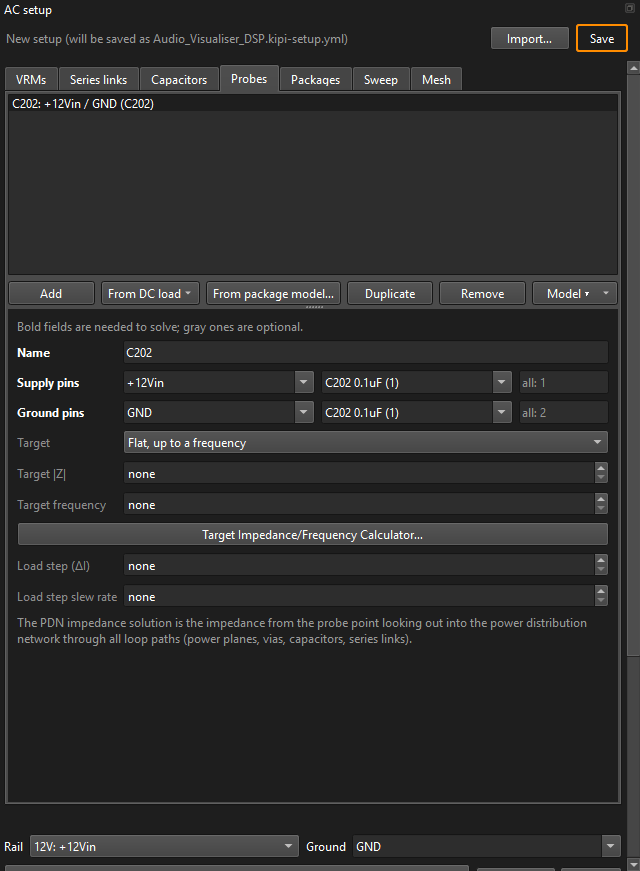
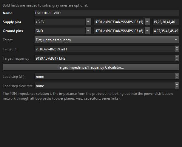
For the dsPIC: Supply pins +3.3V · U701, pins
15,28,36,41,46; Ground pins GND · U701, its ground pins
and exposed pad. (With DC loads in the setup, From DC load copies a load's pins in
one click.)
The target, from the calculator
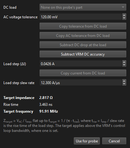
The target impedance is the AC voltage the supply may move by, over the current step that moves it: Ztarget = VAC / ΔI, flat up to ftarget = 1 / (π · trise). Click Target Impedance/Frequency Calculator… and enter:
- AC voltage tolerance 120 mV: the share of the dsPIC's 3.0 to 3.6 V range set aside for ripple and transients, after the regulator's DC accuracy and the DC drop. With a DC solve and DC loads in the setup, the Copy and Subtract buttons work this out from them.
- Load step 0.0426 A: its whole current, switching on.
- Slew rate 12.3 A/µs: how fast it steps.
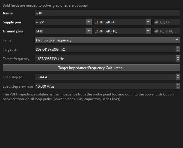
The two LED panel connectors get probes too, on the 12 V rail: each steps by its whole 1.944 A at 10 A/µs and may move by its ±5 % (600 mV), so 600 mV / 1.944 A = 309 mΩ up to 1.64 MHz. With a load step and slew rate entered, the solve also estimates the rail's transient response at the probe.
Check the Sweep and Mesh tabs
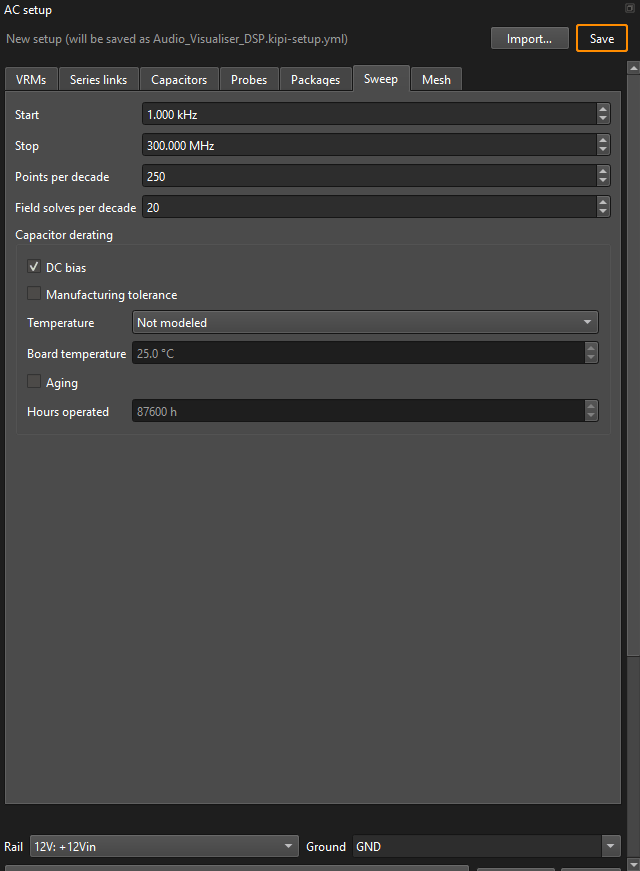
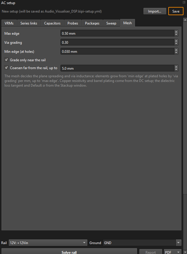
Sweep sets the frequencies: 1 kHz to 300 MHz, 250 points per decade, the copper field-solved 20 times per decade. Under Capacitor derating, DC bias is on, so each model with a voltage rating loses capacitance at its rail's voltage; tick Manufacturing tolerance, Temperature or Aging for a worst case. The Mesh tab's defaults suit most boards.
Solve a rail
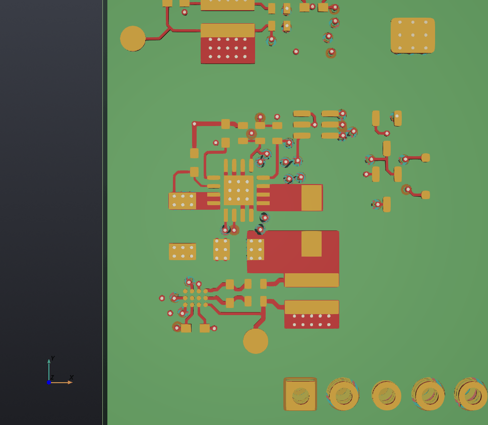
An AC solve covers one rail against one ground. Under the tabs, pick Rail +3.3V (listed by its VRM) and Ground GND, then click Solve rail. The Board map tab comes to the front while it solves, and fills in: the rail's copper over its ground, the probes as red stars and each capacitor as a dot in its model's colour.
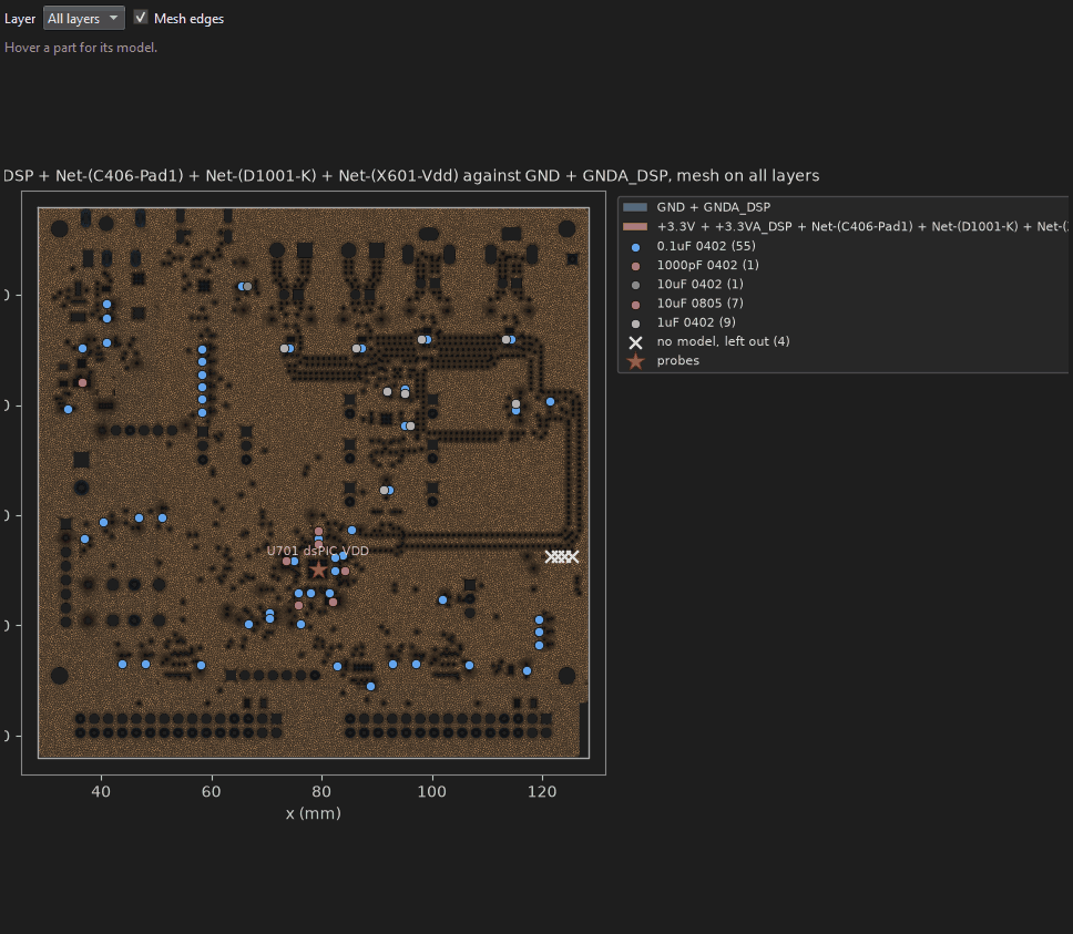
This rail is a big one: its mesh against the ground is 2.5 million unknowns, and its 111 field solves took 19 minutes here. The log counts them down.
Read the impedance curve
The Impedance tab plots |Z| against frequency: the probe's curve, solid, and its target, dashed, from the VRM's bandwidth (the dotted line at 50 kHz) to the target frequency.
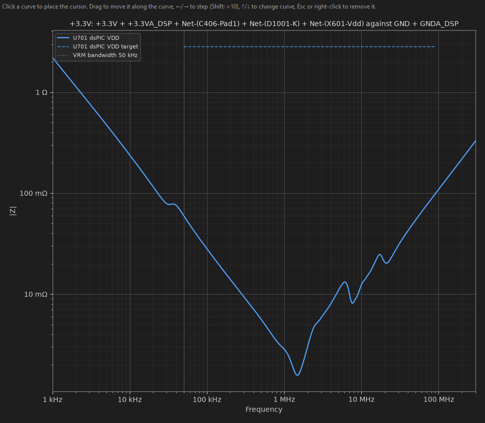
Reading it left to right:
- Falling at −20 dB/decade up to about 1 MHz: capacitive. Below 50 kHz this is the open-loop curve the regulator's loop would flatten; the target ignores it.
- The dip near 1.5 MHz, 1.6 mΩ: the 10 µF capacitors' series resonance, their capacitance against their ESL and mounting.
- The bumps near 6 and 10 MHz: anti-resonances between the capacitor banks (10 µF, 1 µF, 0.1 µF), where one bank's inductance rings with the next one's capacitance. This is where a tight target usually fails.
- Rising at +20 dB/decade above 20 MHz: inductive. The capacitors' ESL plus their pads, vias and the planes' spreading inductance.
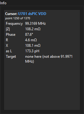
Click the curve to place a cursor; drag it or use the arrow keys. The Info box on the left reads the point: frequency, |Z|, phase, R, X, the equivalent L or C, and the target there with its margin.
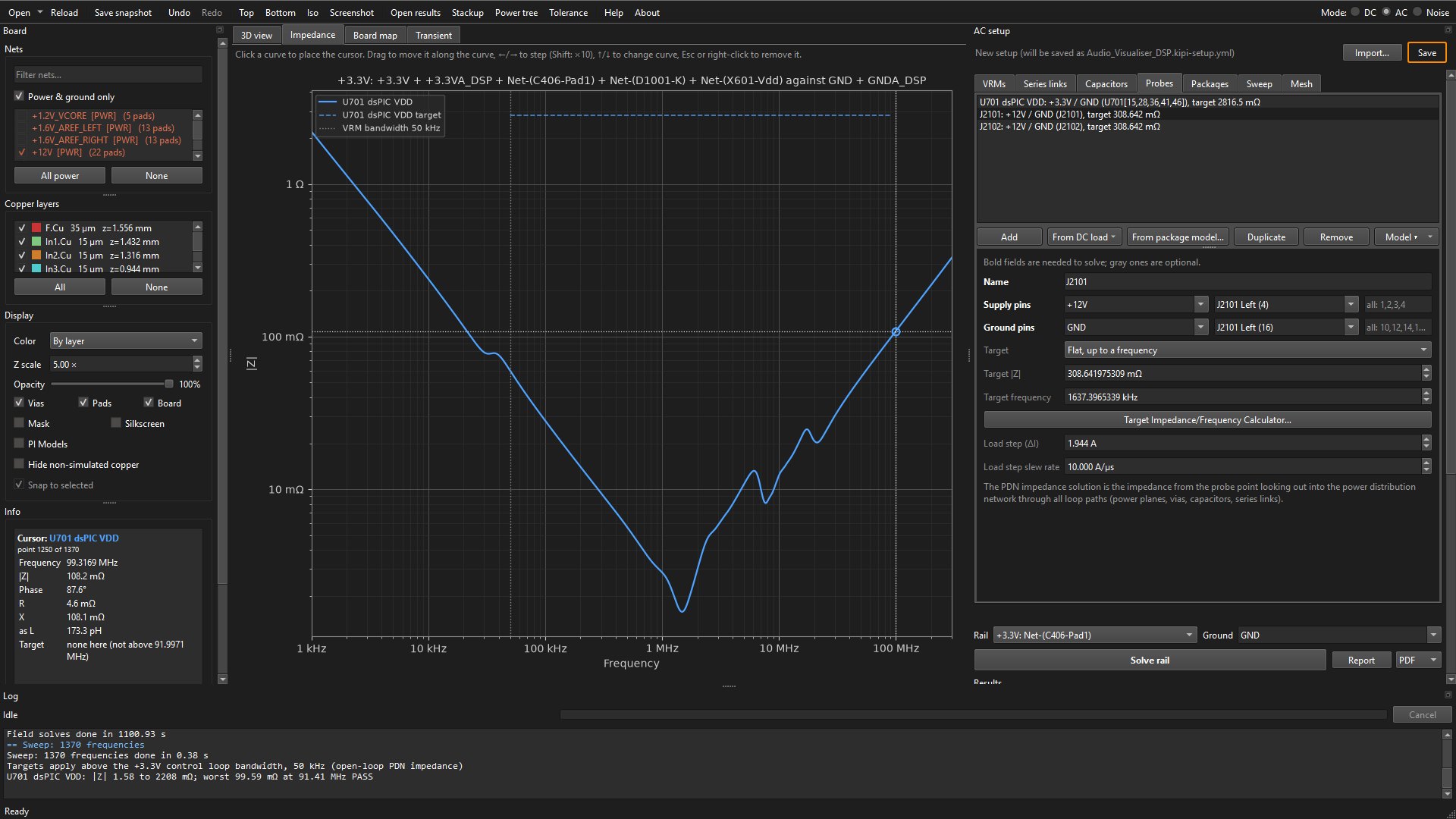
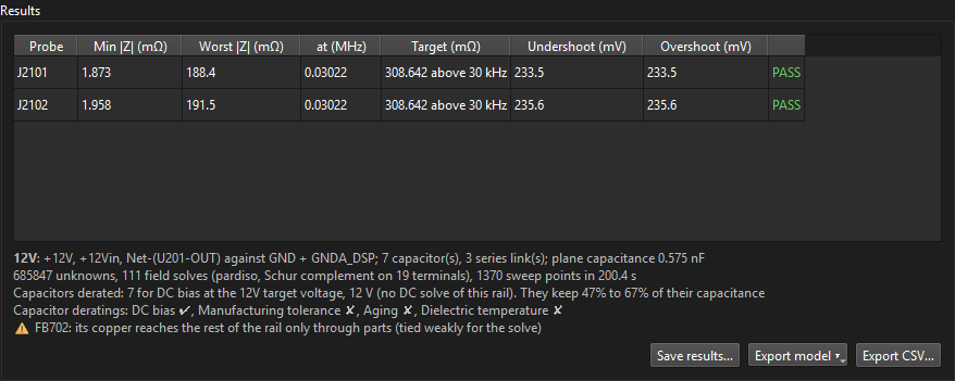
The Results table under the setup gives each probe's lowest and worst |Z| against its target, and the notes below it say what the solve included:
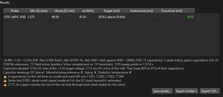
Net-(D1001-K),
behind the diode. That net is solved with the rail because the D1001 link joins it, but it
was never ticked in the Nets list, and the Capacitors table only lists capacitors whose
pads are all on ticked nets, so they could not be given a model. The fix: tick
Net-(D1001-K), give the four parts their models (Tick same value +
footprint) and solve again. Here they sit behind a diode carrying almost no current and
barely touch the dsPIC's curve. The other warnings say how the diode was modelled without a
DC solve of this rail, and that C711's copper reaches the rail only through parts.Solve the 12 V rail and read its transient
Each rail keeps its own result, so switch Rail to 12V and click Solve rail again; switching back shows the +3.3V curves without solving. The 12 V rail is smaller (0.69 million unknowns) and took three and a half minutes.
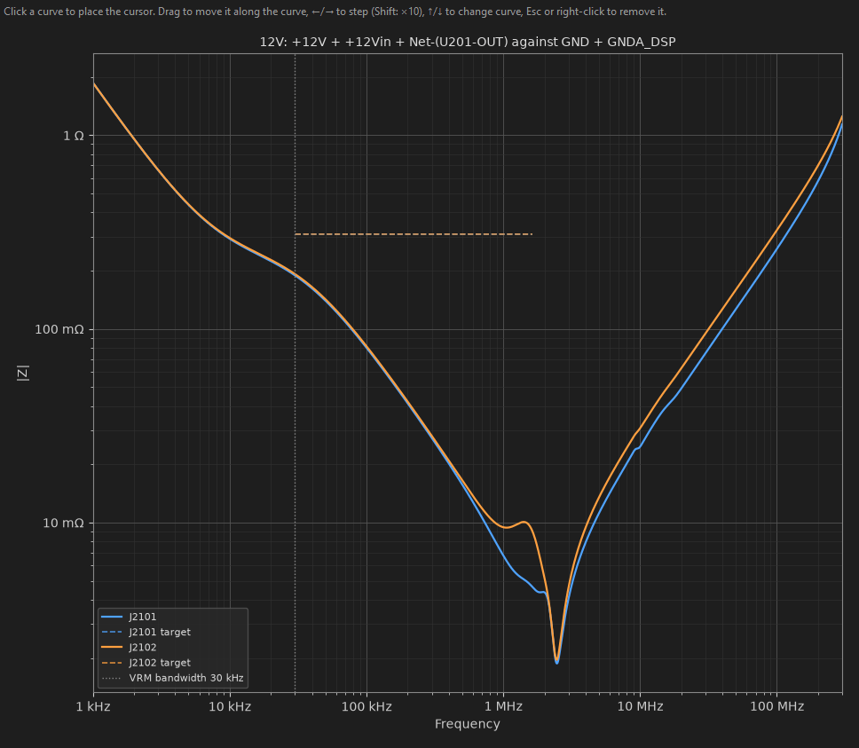
The probes have a load step, so the Transient tab estimates what the rail does when each panel switches on its whole 1.944 A at 10 A/µs, holds, and switches off. The top plot is the load current; the lower one the rail's deviation, against dashed lines at ± target × ΔI (the 600 mV the target stands for).
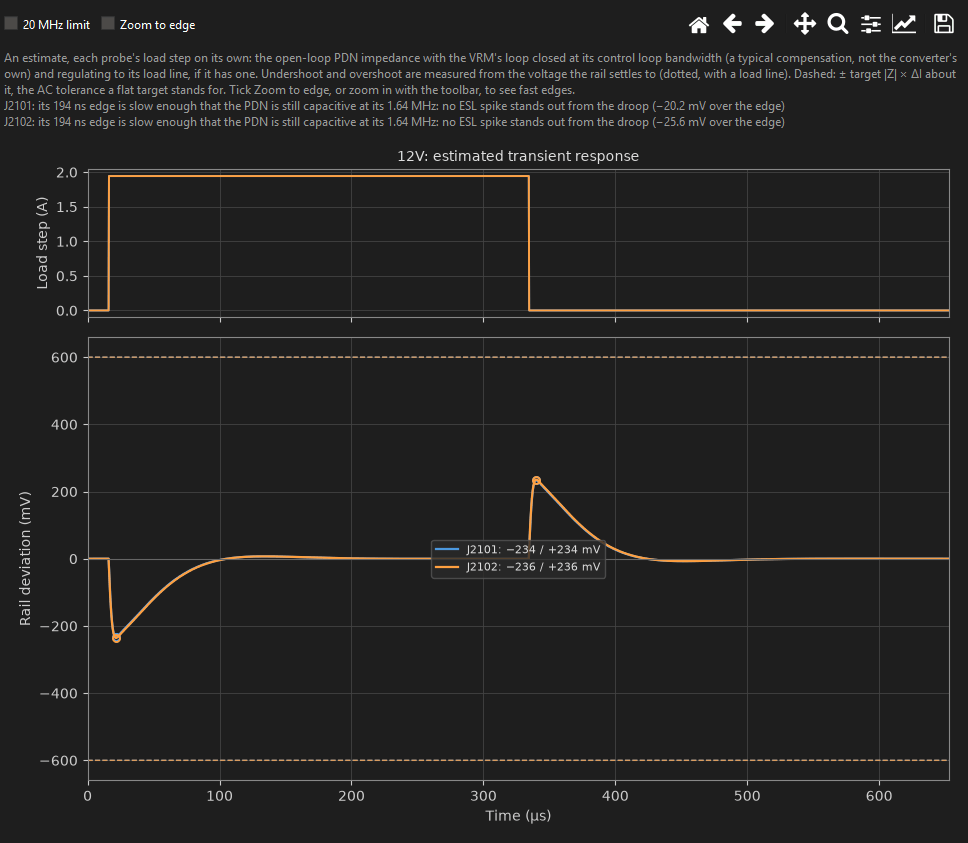
The estimate closes the regulator's loop at its Control loop bandwidth with a typical compensation, so the slow part (the recovery) is approximate and the fast part (capacitors, planes, vias) comes from the solve. Tick 20 MHz limit to see it as an oscilloscope with its bandwidth limit on would.
- Report beside Solve rail writes the shown rail's HTML or PDF report: the probe table, an interactive impedance plot with each capacitor model's own curve, the board map, the transient and the notes (details).
- Save results… keeps every rail solved so far, for Open results…; Export model writes a probe's impedance as a Touchstone or HyperLynx file.
When a probe fails: place the cursor on the worst point. A peak between two dips calls for more capacitance between the two banks, or more damping (ESR); a rising inductive slope for lower-ESL parts closer to the pins and more vias; a failure just above the loop bandwidth for more bulk capacitance.
Part 3: Switcher noise on signals (Coupled Noise)
A buck converter switches its input on and off a few million times a second. Its switch node swings from 0 to 12 V in a couple of nanoseconds, and its hot loop (input capacitors, high-side switch, low-side switch and back) carries current pulses with edges just as fast. Both reach the traces nearby: the switch node's dV/dt through their mutual capacitance (capacitive coupling), the hot loops' dI/dt through their mutual inductance (inductive), and the switching current's return through shared ground copper (common ground). Coupled Noise builds the converter's waveforms from the layout, couples them onto the signals you name, the victims, and compares the noise at each receiver with its noise margin.
On the DSP board the aggressor is the TPS62150A buck, U402, making +3.3V from 12 V at
2.5 MHz. Right beside it runs its own power-good line, Net-(U402-PG), to the
74LVC1G97 gate U401: an open-drain signal held high by a 10 kΩ pull-up, about as easy to
disturb as a logic line gets. Is it safe?
What it needs, and switching to Noise
Coupled Noise reads the rest of the setup: an aggressor is made from a VRM of type Switcher, so the VRMs come from DC or AC mode (the Noise setup has no VRMs tab). It also uses the series links and the capacitor models, and an AC probe if you want the ripple at a chip's pins. So this part starts from the VRMs, series links, capacitor models and dsPIC probe of Part 2, with nothing in its own tabs yet. (Starting truly fresh: add the switcher VRM in DC or AC mode first, as in Part 1.)
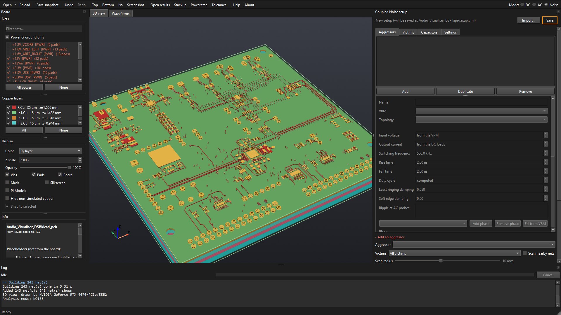
Click Noise beside Mode (or press Ctrl+3). The setup becomes the Coupled Noise setup, with Aggressors, Victims, Capacitors and Settings tabs, and a Waveforms tab appears beside the 3D view. Keep the same nets ticked: the board model solves the converter's input and output rails and their ground.
Add the aggressor
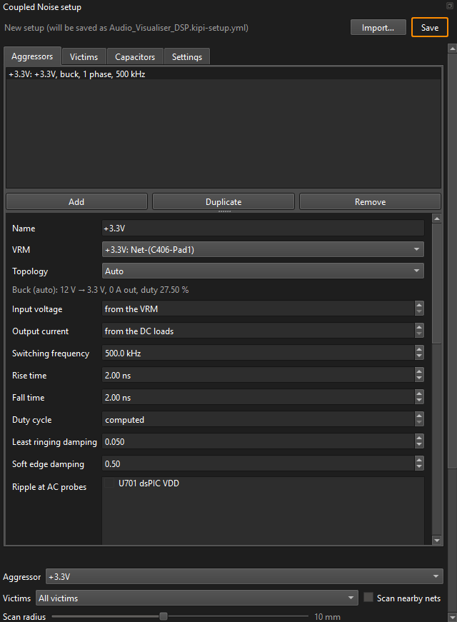
On the Aggressors tab click Add. KiPI makes an aggressor for the first switcher VRM and fills its phase from the board: the inductor between the switching device and the rail, its value, the switch node, the device's pins on each side, and every capacitor from the input and output rails to ground. The line under Topology shows the operating point it worked out: Buck (auto): 12 V → 3.3 V.
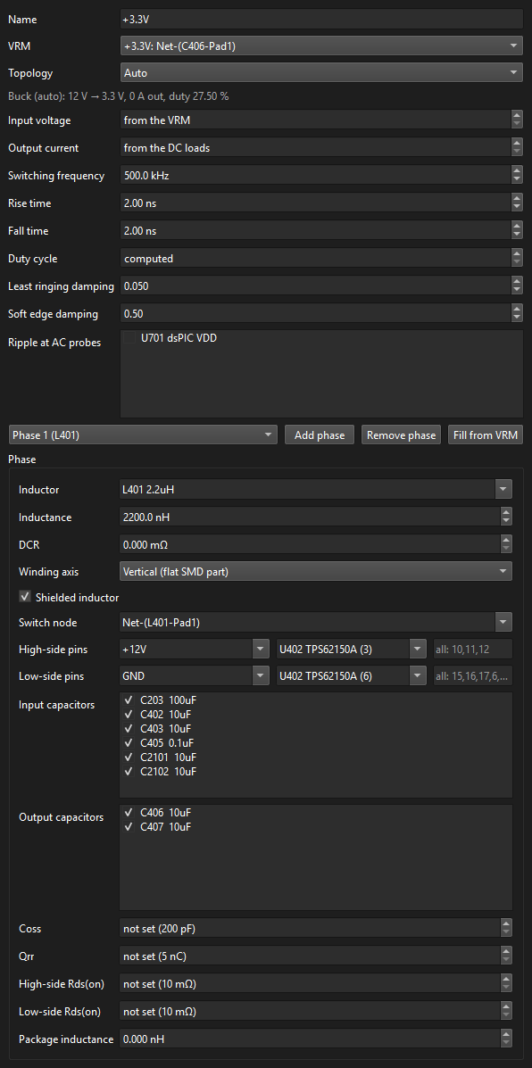
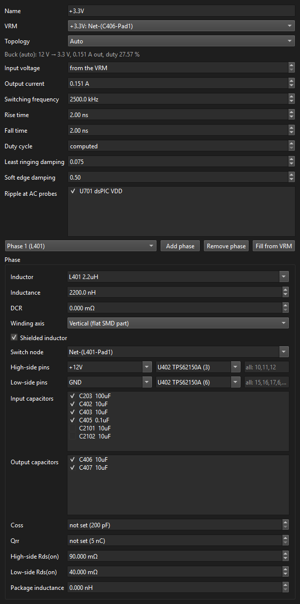
Work down the form with the TPS62150A datasheet and the schematic:
| Field | Value | Where it comes from |
|---|---|---|
| Output current | 0.151 A | What +3.3V's loads draw: the sum of the DC loads on the rail from Part 1. With DC loads in the setup, from the DC loads does this by itself. |
| Switching frequency | 2500 kHz | The TPS62150A's 2.5 MHz mode (its FSW pin tied low). |
| Rise time, Fall time | 2 ns | The switch node's edges. Datasheets rarely give them; 1 to 5 ns is typical for an integrated buck, and a scope on the switch node tells you exactly. Faster edges reach higher frequencies and couple more. |
| Least ringing damping | 0.075 | Real switch nodes ring for five to ten cycles. The default 0.05 is on the pessimistic side of that; 0.075 is a little less. If you can, measure it: scope the switch node and count the cycles. |
| Ripple at AC probes | U701 dsPIC VDD | Tick the AC probe to see the buck's ripple at the dsPIC's pins. |
And in the Phase box below:
- Inductor L401, 2.2 µH. It is a shielded, flat SMD part: Winding axis Vertical and Shielded inductor ticked, so its stray field is the small one a shield lets out.
- Switch node
Net-(L401-Pad1); High-side pins U402 on+12V(its VIN pins); Low-side pins U402 onGND(its ground pins). Add found these from the VRM's pins. - Input capacitors: untick C2101 and C2102. They are on 12 V, but at the LED panel connectors across the board; the buck's hot loop closes through the capacitors beside it, C203, C402, C403 and C405. Output capacitors: C406 and C407. The ticked ones are the phase's own hot loops, traced and coupled as such; with the board model on, the switching current still divides among every capacitor on the rails through the copper, so C2101 and C2102 carry their share and show in the plots.
- High-side Rds(on) 90 mΩ and Low-side Rds(on) 40 mΩ, from the datasheet's electrical characteristics. They damp the ringing and set the conduction losses. Coss and Qrr are not given for an integrated buck; the typical values (shown in brackets) stand in.
Add the victim
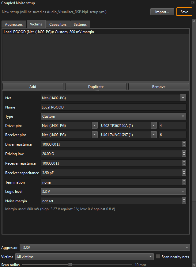
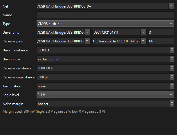
On the Victims tab click Add. KiPI picks the first signal net that is not a victim yet and guesses its driver and receiver as the net's two pads farthest apart:
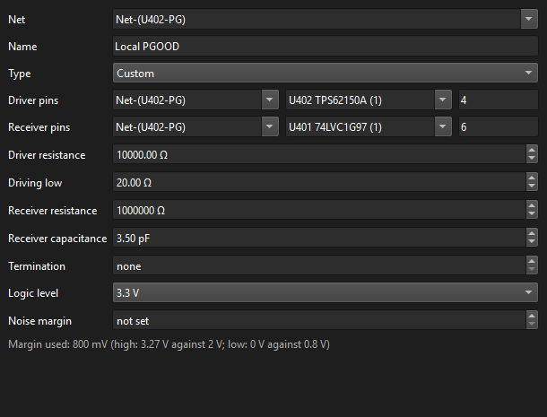
For the power-good line:
- Net
Net-(U402-PG), Name Local PGOOD. - Driver pins U402 pin 4 (PG); Receiver pins U401 pin 6, the gate's input.
- Type: start from Open drain, pulled up. PG is an open-drain output: high it is held only by its pull-up, low by its switch (Driving low 20 Ω). The preset assumes 4.7 kΩ; this board's pull-up is 10 kΩ, so set Driver resistance to 10000 Ω, which makes the type Custom.
- Receiver resistance 1 MΩ and Receiver capacitance 3.5 pF: the 74LVC1G97's input, from its datasheet.
- Logic level 3.3 V. With Noise margin not set, KiPI takes JESD8's 3.3 V CMOS thresholds, VIH 2 V and VIL 0.8 V: 800 mV of margin, the smaller of the two gaps (line 3.27 V high against 2 V, 0 V low against 0.8 V).
With PI Models ticked under Display, the driver and receiver are marked in orange in the 3D view; clicking a marker selects its victim.
Check the Capacitors and Settings tabs
The Capacitors tab is AC mode's, with the same models. Every capacitor the aggressor uses should have one: a capacitor without a model is taken at its board value with a typical ESR and ESL, and the results say so.
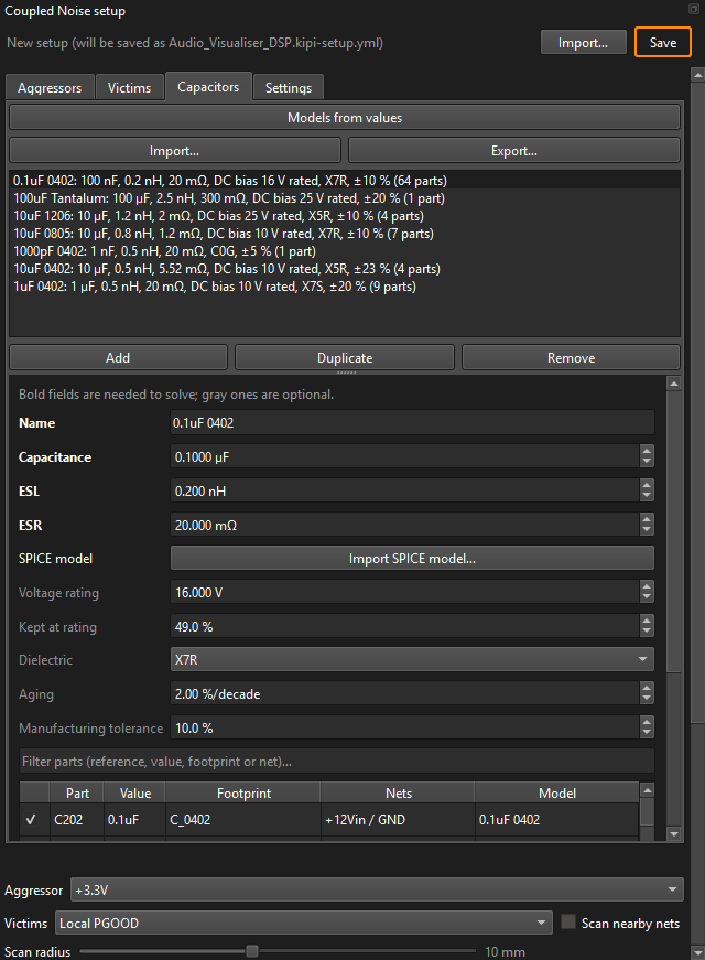
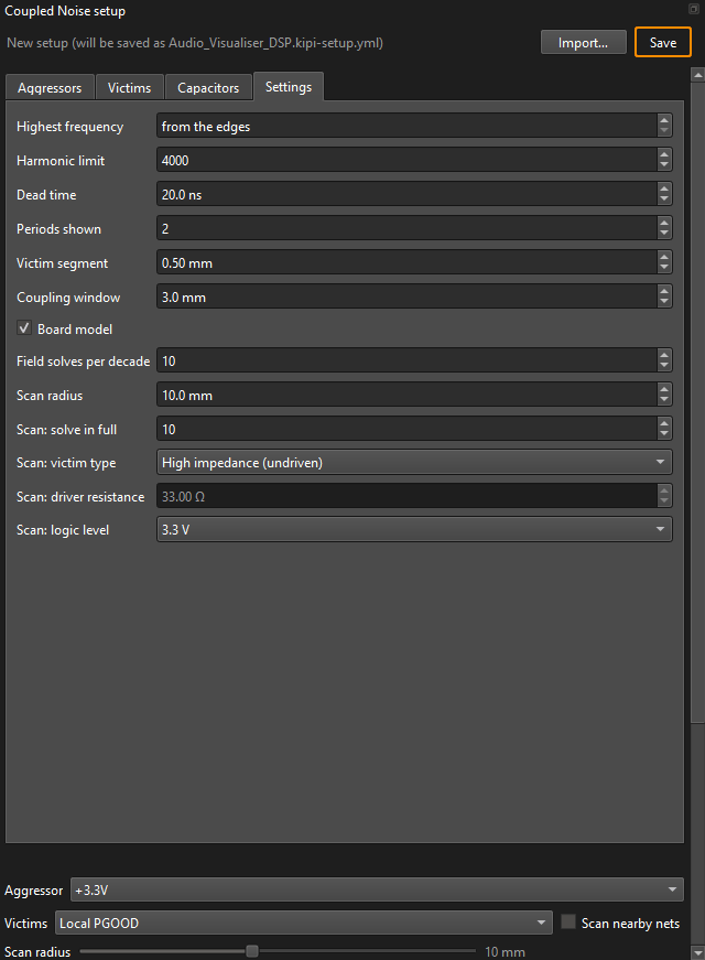
The defaults in Settings suit most boards. The ones worth knowing:
- Board model: solves the 12 V and +3.3V rails and ground with AC mode's field model, so the switching currents divide among the capacitors through the copper, each hot loop is traced through the real copper and vias, and the ground difference between a victim's ends gives its common-ground noise. It is the slow part of a solve; untick it for a quick look while you move parts around.
- Victim segment and Coupling window: victims are cut into 0.5 mm pieces, each with its own cross-section of the copper within 3 mm of it.
- Scan radius and the Scan: fields: for scanning the nets around the aggressor.
Solve the aggressor
Below the tabs, Aggressor is +3.3V and Victims All victims (or one by name, quicker while you rework one route). Click Solve. With the board model on this is about as slow as an AC solve of the two rails: 2.35 million unknowns and 30 field solves, eight and a half minutes here. The waveforms themselves are exact Fourier series and take well under a second, so with the board model off a solve is quick.
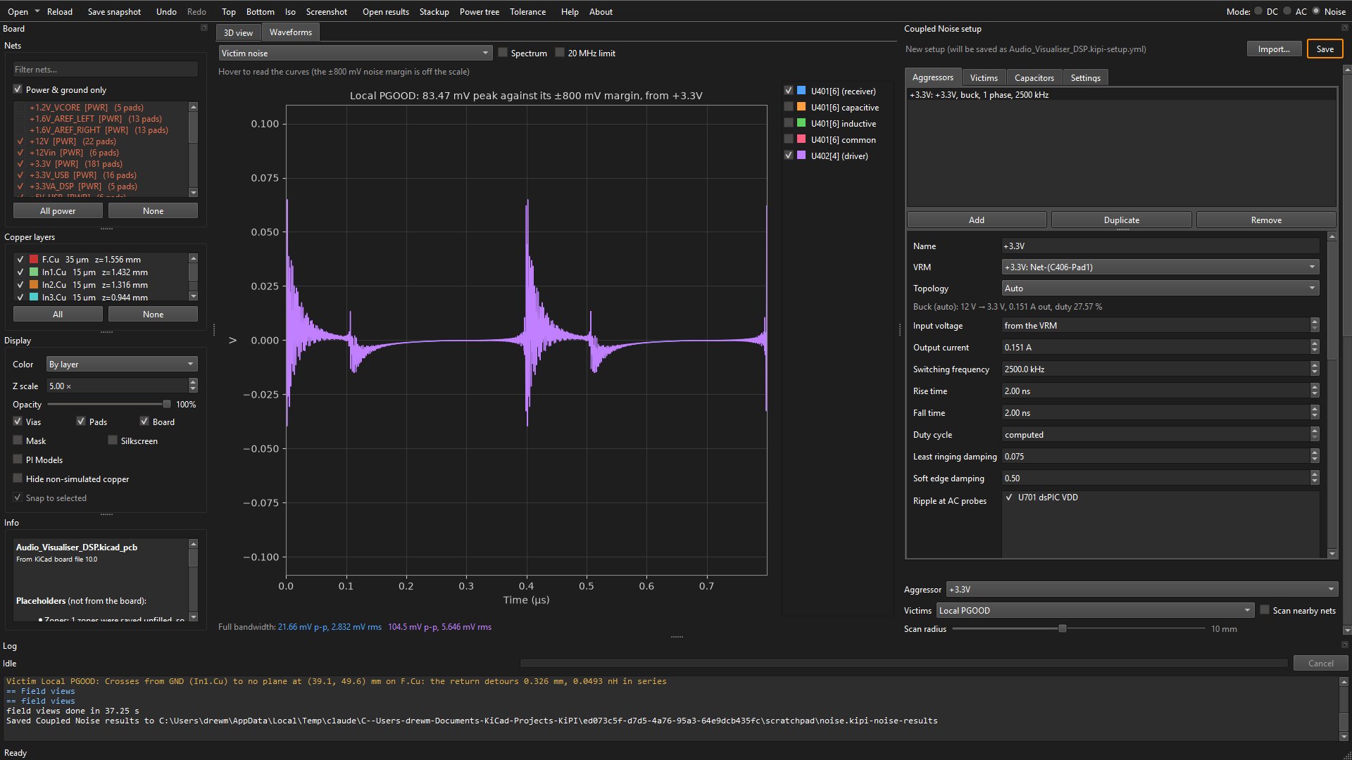
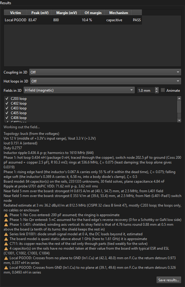
Start with the Results table and its notes:
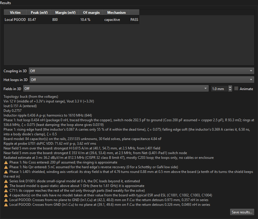
Each victim's row gives its receiver's peak noise over a switching period, its margin, the share of the margin used, the mechanism that dominates, and the verdict. The notes say how the converter was modelled; read them top to bottom:
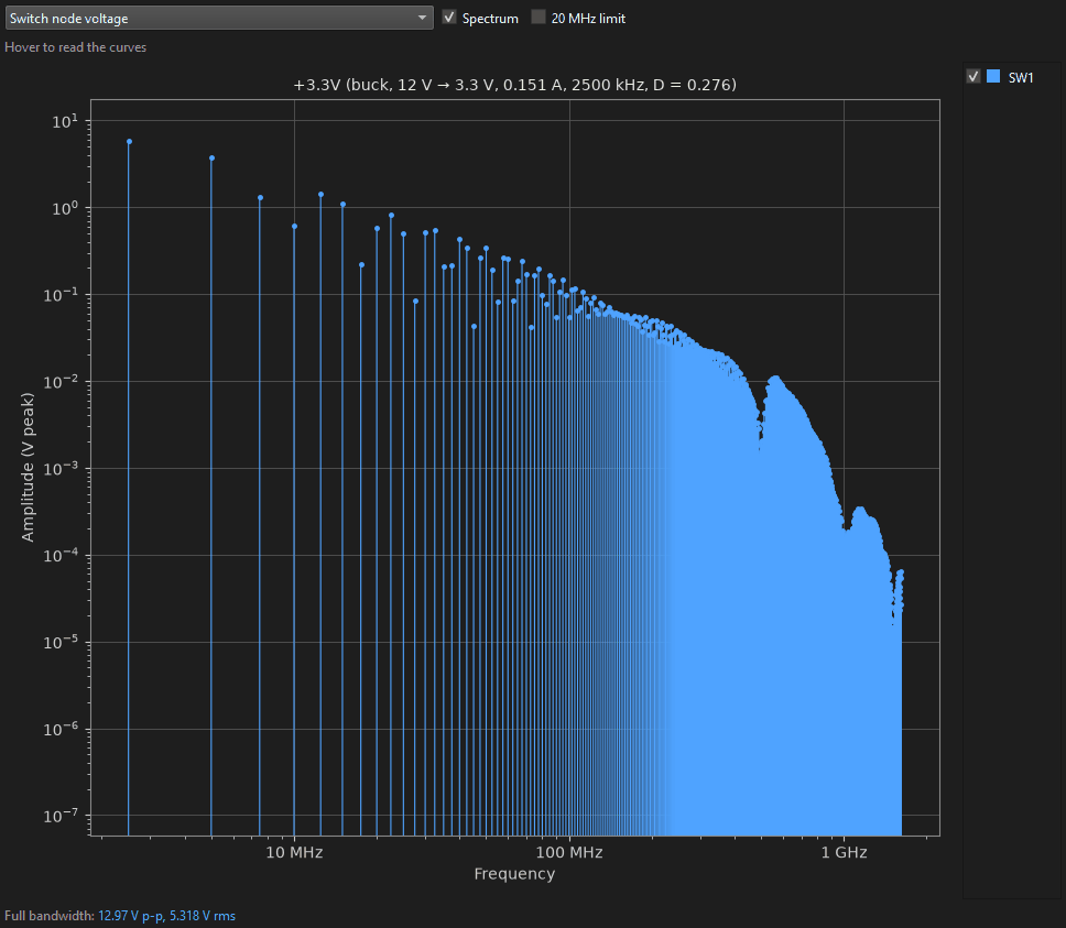
- The operating point: buck from 12 V to 3.3 V, 0.151 A, duty 0.276, and 0.436 A p-p inductor ripple. Harmonics up to 1.61 GHz (644 of them), set by the 2 ns edges and the ringing.
- The hot loop: 0.434 nH, traced through the copper; the switch node's 202.5 pF to ground (the 200 pF Coss assumed plus 2.5 pF of copper); ringing at 537 MHz. A smaller loop has less inductance, so it rings higher and with less energy: this is the number a tighter layout improves.
- The edges: the rising edge is hard. At this light load the inductor's 67 mA valley current carries the node only 55 % of the way within the 20 ns dead time, so the high side finishes the edge and the node rings. The falling edge is soft, carried by 0.369 A into the low side's body diode, which damps it.
- The board model: 84 capacitors on the rails, 30 field solves, 4.84 nF of plane capacitance; and the dsPIC probe's ripple, 71.6 mV p-p.
- Near field and a radiated estimate: where a near-field probe 5 mm over the board would find the strongest H field (at L401) and E field (over the switch node), and a first estimate at 3 m against CISPR 32 class B: 36.2 dBµV/m at 812.5 MHz against 47, mostly from C203's loop. It counts the board's loops only, no cables or enclosure: an indicator of which loop radiates, not a compliance result.
- Warnings: the assumed Coss and Qrr (enter them where a datasheet gives them); L401's shielded stray field; D1001 biased without a DC solve; C1001 to C1004 still without a model (as in Part 2); and two places where PGOOD crosses the edge of the ground plane on In1.Cu, with the inductance each detour adds.
Read the waveforms
The Waveforms tab plots two switching periods of each quantity; pick one in the menu at the top left. Hover to read a curve, and untick a curve's box on the right to hide it. The footer gives each curve's peak-to-peak and RMS.
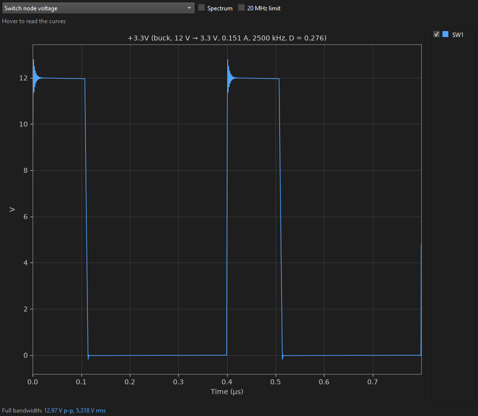
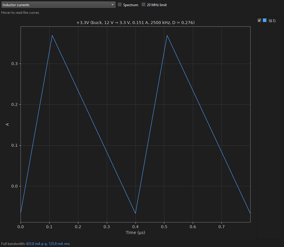
The inductor current dips below zero because KiPI models the buck in continuous conduction. At light load many bucks, the TPS62150A among them, switch to a power-save mode that skips pulses instead. For a worst case the continuous waveform, with its fast edges every period, is the right one to check.
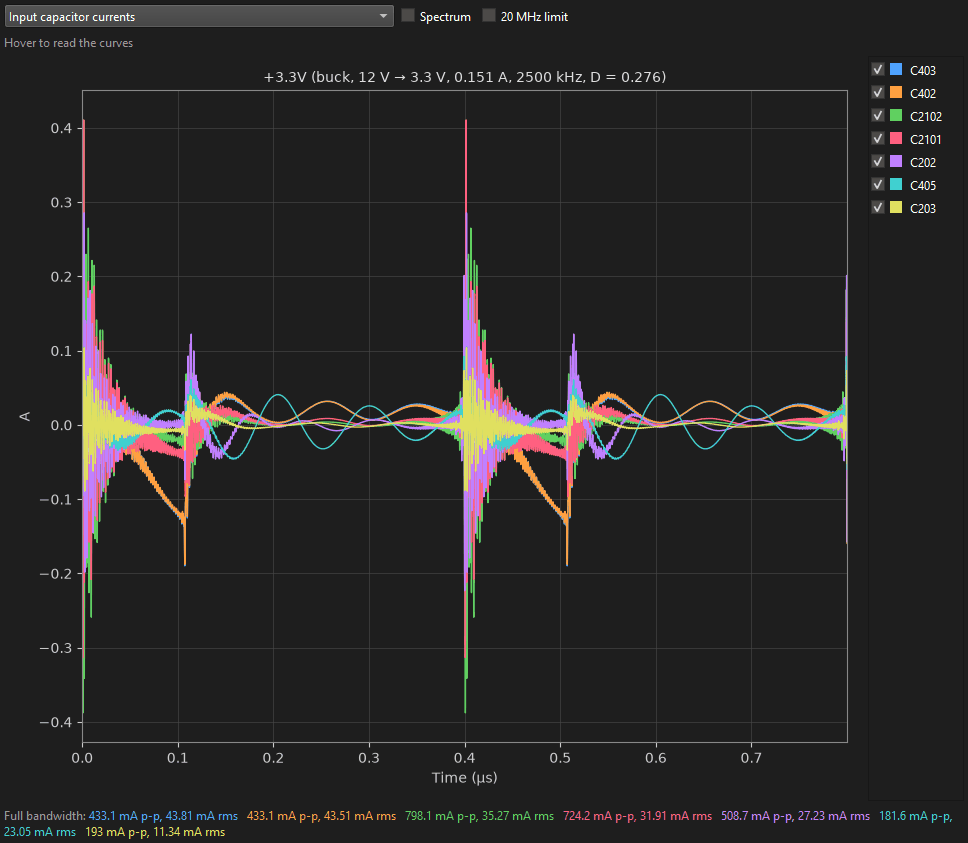
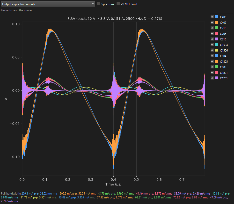
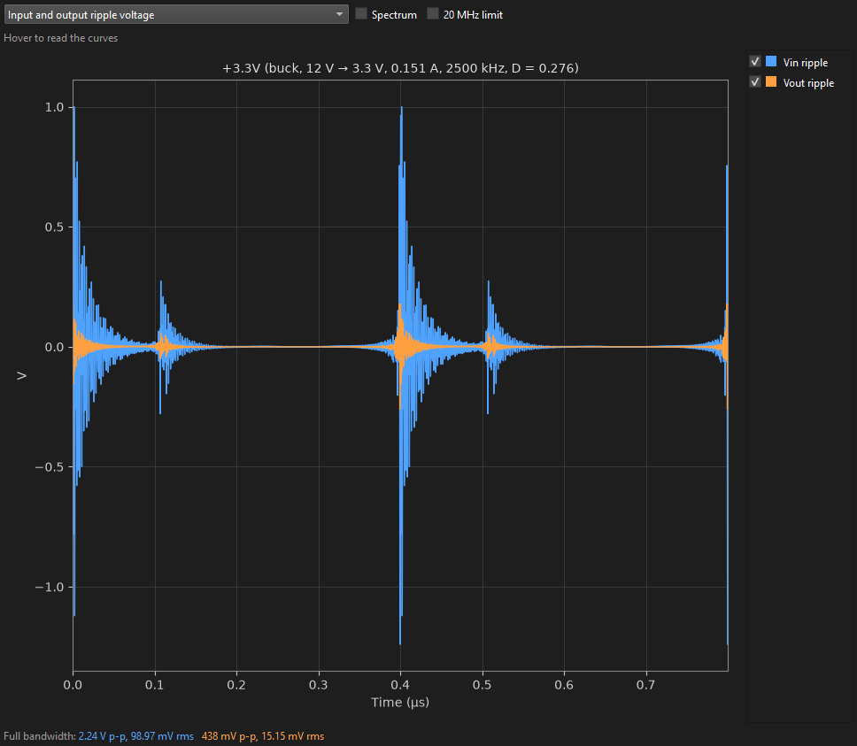
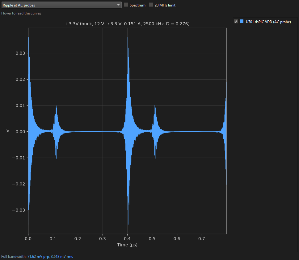
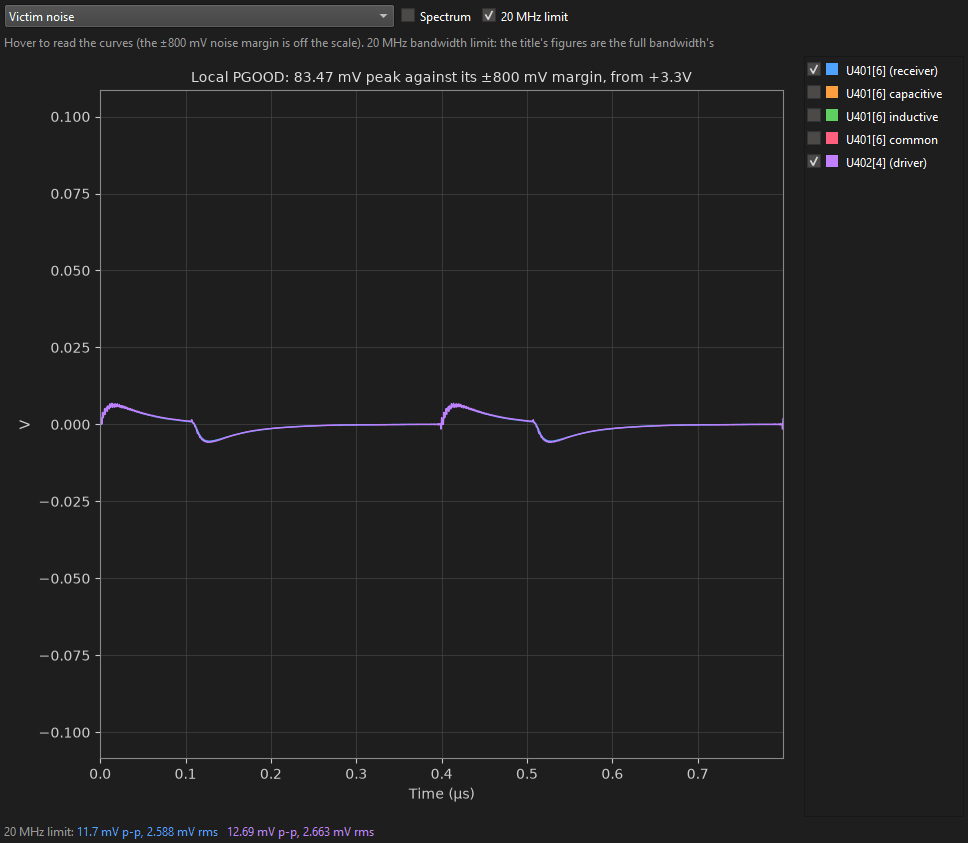
Spikes that big look alarming, but they last a nanosecond or two. Tick 20 MHz limit to see any view as an oscilloscope with its bandwidth limit on would (the usual way ripple is specified); the titles and the table keep the full bandwidth's figures. Tick Spectrum to see the harmonics instead:
The victim's noise
Victim noise plots the selected victim's noise at its receiver and at its driver end. Tick Capacitive, Inductive or Common to add each mechanism's own curve. Victim held high and low plots the line as it sits, with the noise on it, against VIH and VIL:
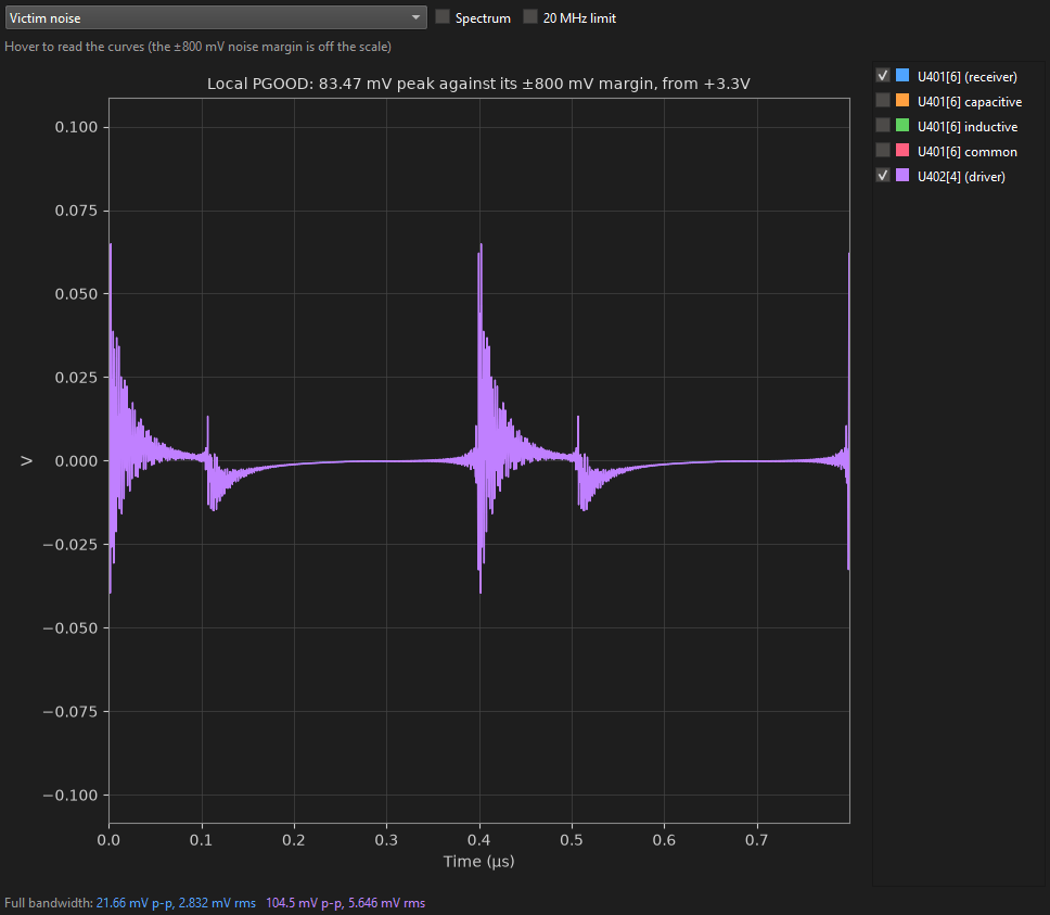
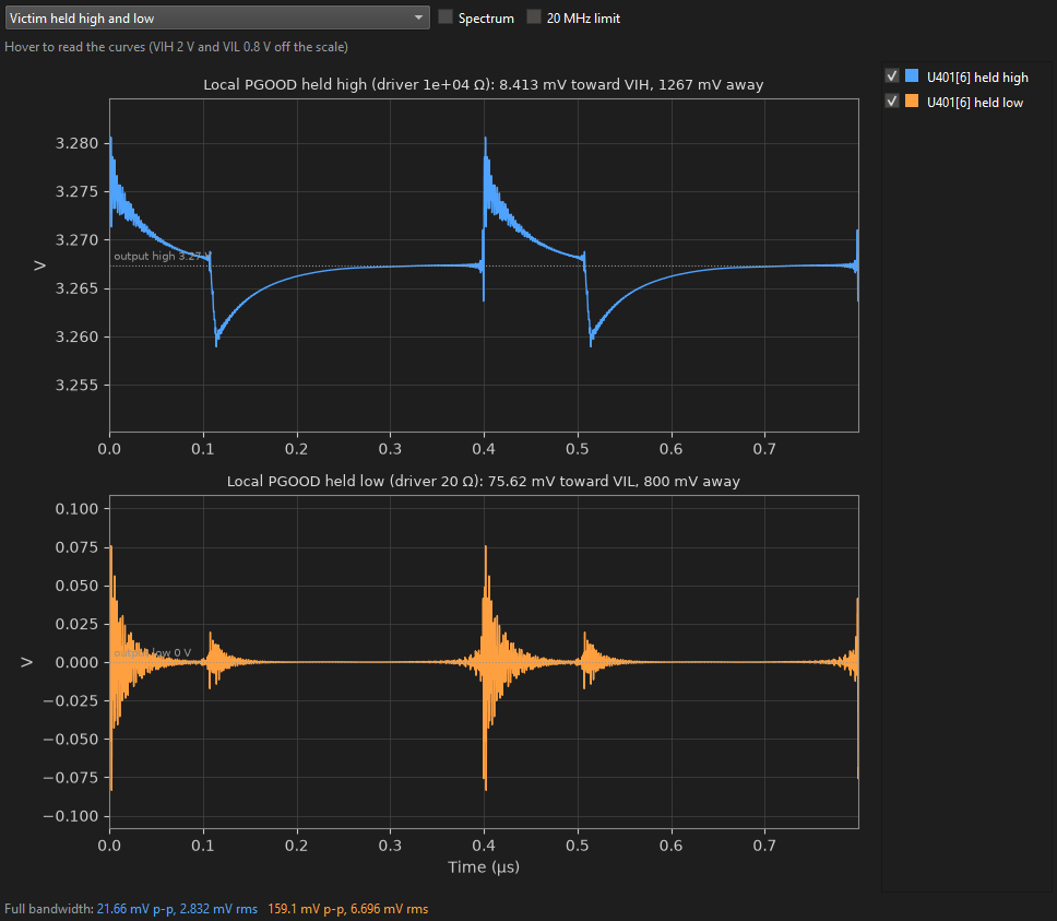
An open drain is solved in both states because its driver differs: the 10 kΩ pull-up high, the 20 Ω switch low. The verdict takes the larger noise of the two against the smaller margin: 83.5 mV of 800, a comfortable PASS. A victim using more than about half its margin deserves a closer look, and a FAIL a layout change (see where the noise comes from).
See where the noise comes from
Three menus under the results table draw the solve in the 3D view (click the 3D view tab). They answer the question a FAIL leaves: what to move.
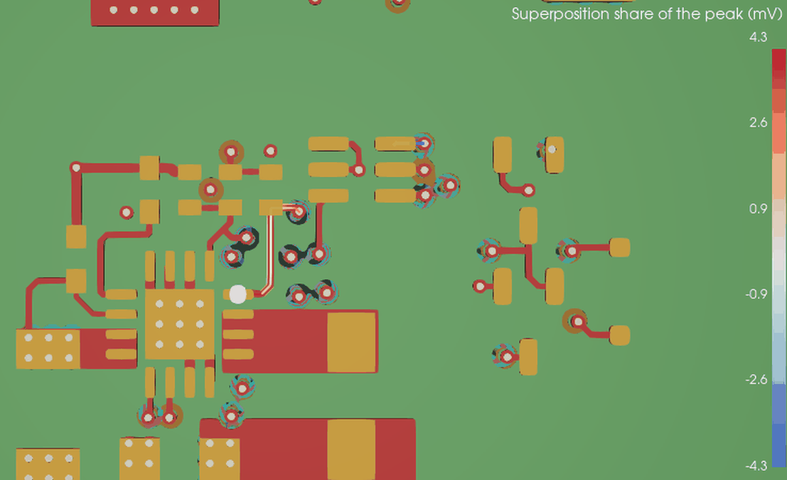
Coupling in 3D
Pick Superposition (or one mechanism). Each piece of the selected victim's trace is coloured by its share of the receiver's peak: red adds to it, blue takes from it, and the shares add up exactly to the peak. The common-ground share is a dot at the driver. The brightest pieces are the ones to reroute.
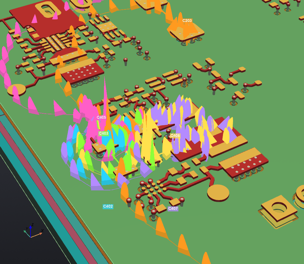
Hot loops in 3D
Pick All capacitors, or one. Each capacitor's loop is drawn as streamlines of the current the solve traced through the copper, in its own colour with its name at the capacitor and cones pointing the way the current flows: from its positive pad to the switching device, through it, and back through the ground's copper, vias and plane. Where the lines bunch the current is densest; where they dive down a via and run in the plane, that is where the return really goes. The line under the menu gives each loop's inductance.
Fields in 3D
Pick H field (the current loops and the inductor's stray field) or E field (the switch node's charge) and tick the sources in the list. Each point of a slice over the board, at the height entered, is coloured by its peak over a switching period, with arrows along the field. Tick Animate to play it through one period; click a part or net in the 3D view to add its field.
The mechanisms call for different fixes. Capacitive noise comes from the switch node's dV/dt: keep victims away from the switch node's copper, or behind a plane, and drive them harder (a smaller pull-up). Inductive noise comes from the hot loops' dI/dt: make the loops small, keep them over a solid plane, and route victims away from them or on the far side of the plane. Common noise comes from the switching current's return: give the hot loop its own short return to ground and keep the victim's driver and receiver grounds out of it.
Scan the nets nearby
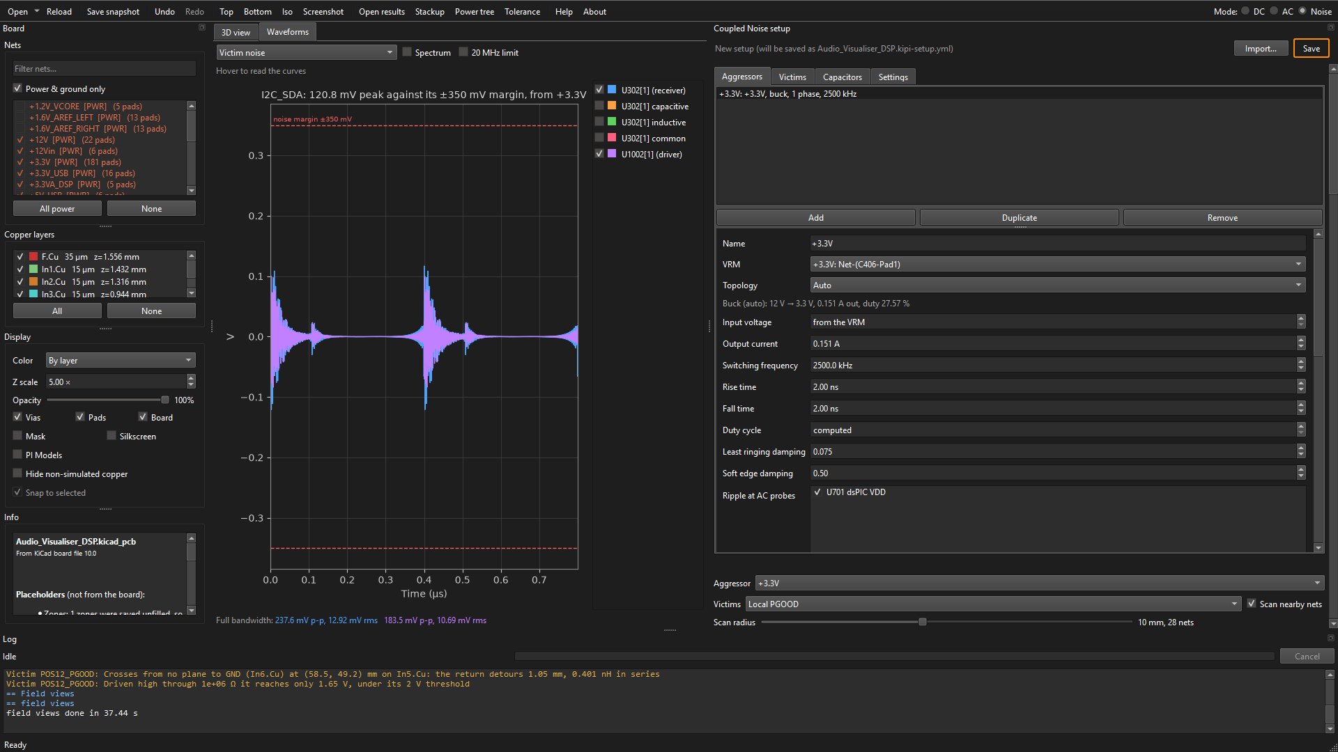
The victims you name are the ones you thought of. To find the ones you did not, tick Scan nearby nets beside Victims and set the Scan radius under it: every signal net with a trace that close to the aggressor's parts gets a quick estimate, and the worst (Scan: solve in full in Settings, 10 by default) are solved in full. 10 mm takes in 28 nets on this board.
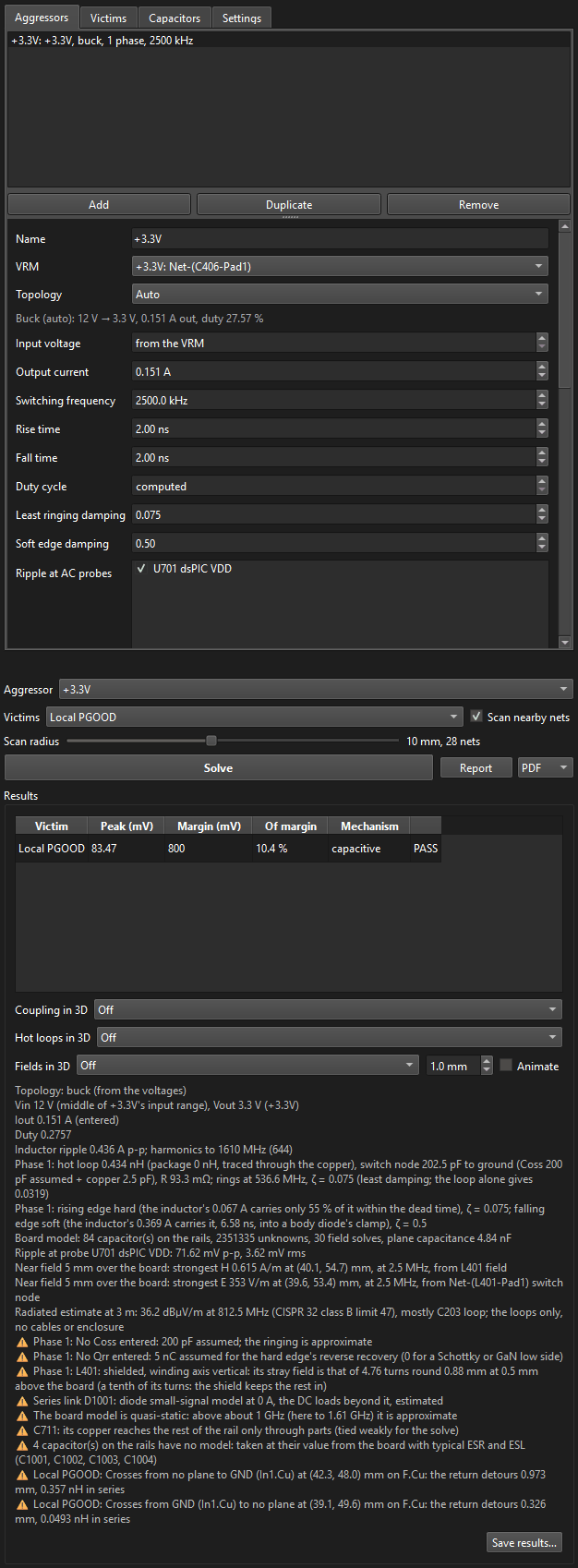
The real drivers of scanned nets are not known, so they are solved as Scan: victim type, High impedance (undriven) by default: a floating line held by nothing but its inputs' leakage, the worst case for capacitive coupling. Its margin is smaller too: undriven, the line sits half way, 1.65 V, and its margin is the 350 mV to the nearer threshold. A named victim keeps its own type. Click Solve again:
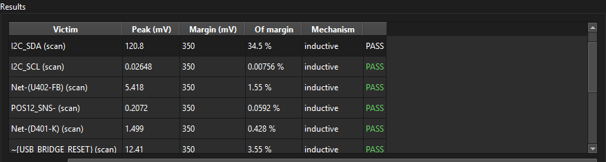
All PASS, even as undriven lines. I2C_SDA comes closest, and inductively: somewhere along its long route it runs close to the buck's hot loops (Coupling in 3D shows where). Held by its real pull-up it would do better than undriven; to check it properly, add it as a victim with its real driver and receiver and solve again. The notes grow long with a scan: each scanned net's plane crossings are listed too.
- Report writes the shown aggressor's HTML or PDF report: the victims against their margins, the parasitics, the waveforms, each victim's noise by mechanism, the scan's estimates and the notes (details).
- Save results… keeps every solved aggressor for Open results….
Putting it together
Each part answered one question. A load's whole voltage budget takes all three: the DC drop (Part 1), the ripple a switcher puts on its rail (Part 3) and the transient a load step causes (Part 2), on top of the regulator's own accuracy. The Tolerance button on the toolbar opens a window that adds them up per load, side by side against each load's DC, AC and total tolerances, from whichever results are loaded, solved or opened from files. On your own board, where the three modes share one setup:
- Give each load a tolerance, and its DC tolerance and AC tolerance where its datasheet splits them (DC setup, Loads).
- Solve DC. Give each load you care about an AC probe on the same pins (From DC load in AC mode) with a load step, and solve its rail.
- In Coupled Noise, tick that probe under the switcher's Ripple at AC probes and solve.
- Open Tolerance, tick the loads, and read each one's PASS or FAIL. Save the table to keep it with the board revision.
The Tolerance stack-up section of the User Guide describes every column.
Where to go next
- The User Guide: every control, every result column, the step-by-step workflows (multi-phase regulators, remote sense, partial solves, decoupling studies) and troubleshooting.
- The Solver Guide: what PI analysis is, and how KiPI's mesh and its DC, thermal, AC and coupled noise solvers work.
- Hover any field in KiPI for its tooltip, and press F1 for the User Guide.