KiPI User Guide
How to set up, solve and read power integrity simulations of a KiCad board. Every section below can be opened and closed; use the contents on the left to jump around.
What KiPI does
KiPI is a power integrity (PI) analyzer that runs as a KiCad 9/10 plugin. It reads the copper of your board straight from the PCB editor and simulates how power gets from your regulators to the parts that use it. It also runs standalone, without KiCad, on board files. It has two analysis modes, chosen at the right end of the toolbar:
New to power integrity? The Solver Guide explains what PI analysis is, why it matters, and how the mesh and the DC, thermal and AC solvers work.
| Mode | Question it answers | What you get |
|---|---|---|
| DC | With every load drawing its current, what voltage actually reaches each pin, how much current flows through each trace, plane and via, and how hot does the board get? | IR drop and PASS/FAIL per load, voltage, current density, power density, via current and temperature maps in 3D, VRM and loss tables, an optional HTML report. |
| AC | Looking into a device's power pins, how does the impedance of the power distribution network (planes, vias, decoupling capacitors) vary with frequency, and is it below the device's target impedance? | |Z| versus frequency curves for each probe point, a cursor to read values off them, and PASS/FAIL against a flat or custom target mask. |
KiPI infers nothing about your power system from the schematic. You tell it where the regulators are, what each load draws, which parts sit in series between nets, and (for AC) which capacitor model each decoupling capacitor uses. The board's copper, layer stackup, vias and pads come from KiCad.
Quick start
DC voltage drop in ten minutes the most common first run
- In KiCad, enable Preferences → Plugins → Enable KiCad API (once).
- Open your board in the PCB editor and click the KiPI toolbar button. KiPI reads the board (refilling zones first) and draws it in 3D.
- In the Nets list on the left, tick the power and ground nets you want to analyze. KiPI pre-ticks a guess the first time.
- In the PI setup panel on the right, VRMs tab: click Add, pick the regulator's output net and part, set its voltage. Add its Ground pins if you want the ground return solved too.
- Loads tab: click Add for each part that draws current, pick its supply pins, enter its current and a tolerance (e.g. ±3 %).
- If a sense resistor, ferrite, fuse or load switch sits between two nets you ticked, add it on the Series links tab.
- Click Solve all. Watch the log at the bottom.
- Read the Loads table for PASS/FAIL, and click around the 3D view to probe voltages. Switch the field to Current density and tick Arrows to find bottlenecks.
The setup is saved next to your board as <board>.kipi-setup.yml every
time you solve, so the next session starts where you left off.
AC impedance of one rail after the DC setup has a VRM on the rail
- Switch Mode (right end of the toolbar) to AC. The setup panel becomes the AC setup; VRMs and series links are shared with DC.
- Make sure the rail's net, its ground and every net its capacitors connect to are ticked in the Nets list.
- Capacitors tab: click Models from values to make one model per capacitor value, then enter each model's ESL and ESR from the datasheet (and check the capacitance).
- Probes tab: click Add. KiPI picks the busiest part on the rail that also has ground pins, which is usually the load. Or click From DC load and pick a DC load: the probe gets that load's supply and ground pins. Set a target impedance, or open the target calculator.
- Under the tabs, choose the Rail (by its VRM) and Ground, then click Solve rail.
- The Impedance tab in the middle shows |Z| against frequency. Click a curve to place a cursor and read the values in the Info box.
Try it without a board of your own
The repository includes an example: a 4-phase 12 V → 0.9 V, 40 A core rail with decoupling and probes already set up. From a development checkout run
python -m kipi examples/multiphase_buck/multiphase_buck.kipi.json.gz
which opens it in standalone KiPI, or open that file with Open… (standalone) or Open snapshot… (the plugin).
The main window
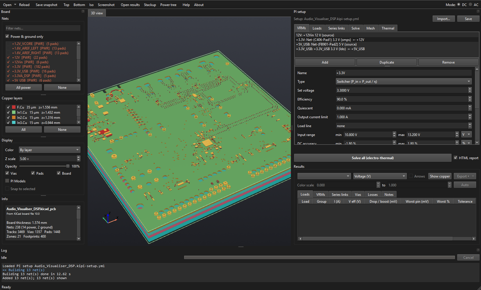
The Board, setup and Log panels are dock widgets: drag their title bars to move them or float them in their own windows.
Starting KiPI
- Plugin or standalone. Started from the KiPI button in KiCad's PCB editor, KiPI
runs as the plugin: it reads the board open in the editor and can re-read it,
refill its zones and select items in it. Started any other way (
python -m kipi, or thekipicommand), it runs standalone: it opens board files with Open… and needs no KiCad. The title bar then ends in (standalone), and the controls that need KiCad are hidden (see the toolbar). Standalone opens KiCad board files (.kicad_pcb), ODB++ jobs and KiPI snapshots (.kipi.json.gz). - KiCad board files. A
.kicad_pcbfrom KiCad 7 to 10 reads the same as the plugin reads it from KiCad, so a board set up in the plugin opens standalone with its setup. Net classes come from the.kicad_pronext to it. KiPI uses the zone fills saved in the file and cannot refill them: fill the zones in KiCad (B) and save before opening. Zones saved unfilled are listed under Placeholders in the board summary. - ODB++. Open a job as a
.zip,.tgzor.tar.gz, or unpacked by picking itsmatrix/matrixfile. KiPI reads the copper as the job gives it and the stackup from its layer matrix. The setup is found by the job's name: exportBoard.zipbesideBoard.kicad_pcbto share the board's setup. Export at 6 decimals if your tool asks: KiCad's default of 2 rounds coordinates to 10 µm. What the job leaves out (copper drawings' nets, a dielectric's thickness) is listed under Placeholders. - Standalone setup. Start standalone KiPI with its launcher:
double-click
kipi_launcher.pyw(Windows) or runpython kipi_launcher.py. The first start installs KiPI's packages into an environment of its own. The setup window lists each package with its size and the totals, and offers PARDISO on Windows and Linux x86-64; nothing is installed until you click Install. Later starts open KiPI straight away. To add or remove PARDISO later, use About → Manage dependencies…: KiPI closes, the setup opens, and KiPI starts again afterwards.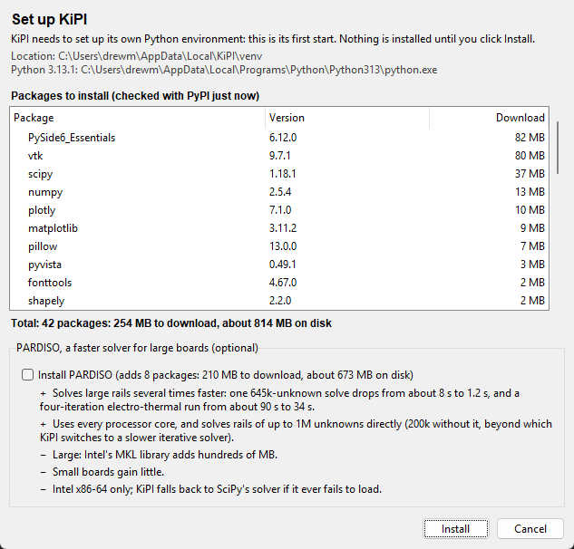
The setup window on a first start. - Pin to the taskbar (Windows): right-click KiPI's taskbar button while it is
open, or its Start menu shortcut (
python kipi_launcher.py --create-shortcut), and choose Pin to taskbar. The pinned button starts standalone KiPI through the launcher, even when it was pinned from the plugin, since only KiCad can start the plugin; a running KiPI of either kind shows on that button. - While KiPI starts it shows a welcome screen with the logo, its version, whether it runs as the plugin or standalone, and the versions of Python and its main packages. It closes on its own after one play of the animation, or when you click it.
- One KiPI at a time (one plugin and one standalone). Clicking the KiPI button while the plugin is already open brings the open window to the front instead of opening a second one; starting standalone KiPI again does the same for the standalone window. The two never take each other's place. A KiPI that crashed does not block the next one.
- One KiCad at a time. KiPI talks to KiCad through its API, which cannot tell two open KiCads apart, so KiPI will not connect (at start or on Load from KiCad) while more than one KiCad project manager or PCB editor is open. The message names each one with its process ID. See Troubleshooting.
Typing values
A number on its own is in the field's unit. Fields in an SI unit (Ω, F, H, Hz, A, V, W, m)
also take a prefix, with or without the unit, and convert it to the field's unit: in a µF
field, 10n, 10 nF and 0.01 are all 10 nF. A resistance
can be written 2 mOhm, 2mΩ or 4k7. Prefixes are case
sensitive (m is milli, M is mega), and u stands for µ.
Fields in other units (%, °C, A/µs, µΩ·cm) take plain numbers. A field shows its usual number
of decimals, plus more when a small typed value needs them.
Toolbar
Every toolbar button
| Button | What it does |
|---|---|
| Load from KiCad plugin | Re-reads the board from the running PCB editor (after you change the layout) and reloads the saved setup. The nets you have ticked stay ticked. Save the setup first if you have unsaved changes. Only one KiCad may be open (see Starting KiPI). |
| Refill zones plugin | When ticked, KiPI asks KiCad to refill every zone and waits for it before reading. KiPI only sees filled copper, so leave this on unless the fills are already current and the refill is slow. |
| Open snapshot… plugin | Opens a board saved with Save snapshot…. KiCad does not need to be running. |
| Open… standalone | Opens a board file:
a KiCad board (.kicad_pcb), an ODB++ job (.zip,
.tgz, or its matrix/matrix file) or a KiPI snapshot
(.kipi.json.gz).
Its saved setup comes with it, as with Load from KiCad. The arrow beside it lists
the boards opened lately. |
| Reload standalone | Reads the open board file again. When the file is saved (in KiCad, say), KiPI asks whether to read it again by itself. Ticked nets stay ticked. |
| Save snapshot… | Saves the extracted board as
.kipi.json.gz, to analyze later, on another machine, or to attach to a bug
report. |
| Top / Bottom / Iso | Snap the 3D camera to look down on the board, up at its underside, or from an isometric angle. They also bring the 3D view to the front from the Impedance and Board map tabs. |
| Screenshot… | Saves whatever is in the middle as a PNG: the 3D view, the impedance plot or the board map, whichever tab is showing. |
| Open results… | Reopens saved results without solving again. Load the same board first. In DC mode it opens a DC solve saved with Export ▾ → Save results…; in AC mode, the rails saved with the AC panel's Save results…. |
| Stackup | Opens the Stackup window: the board's layers with their thicknesses, εr and copper resistivity. |
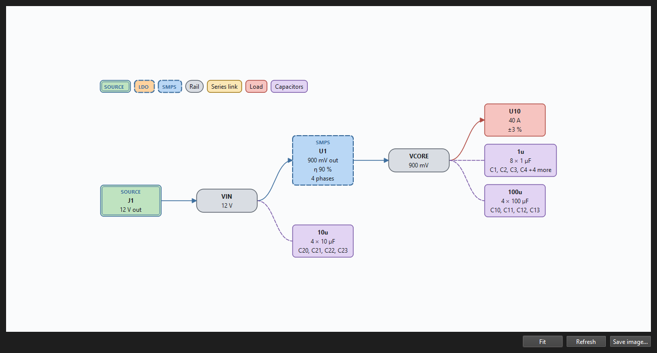
| Power tree | Opens a block diagram of the setup, drawn left to right in the direction power flows: each source and regulator, the rails they drive, series links between rails, and the loads and capacitor models on each rail (capacitors are grouped per model and rail, with a dashed line). VRM types differ in colour and tag: a SOURCE has a double border, and regulators (LDO and SMPS) a dashed one. A rail with three or more loads, or capacitor groups, packs them into a framed grid fed by one arrow, titled with their count (and the loads' total current); the grids take the shape that lets the whole tree fit the window largest. Each block sits just right of the one feeding it. Ground nets, and net ties between them, are left out. Hover a block for its pins; drag to pan, Ctrl + wheel to zoom, Save image… for a PNG. It redraws as the setup changes. |
| Help F1 | Opens this guide in your web browser. |
| About | Version, author and project links, and how often the project has been cloned and its releases downloaded. Those counts are fetched once a session from the project's GitHub repository; offline, the last ones fetched are shown, or none. Copy version info copies the versions of KiPI, Python, its libraries and the sparse solver in use, for bug reports. Check for updates asks GitHub for the newest KiPI release and says whether it is newer than yours, with a link to download it; KiPI never checks on its own. In standalone KiPI started by its launcher, Manage dependencies… closes KiPI and opens its setup (for example to add or remove PARDISO). |
| Mode: DC / AC | Chooses the analysis. The setup dock shows that mode's panel. The DC setup and results are kept while you are in AC and come back when you switch to DC. You cannot switch while a task is running. |
Stackup window
The Stackup toolbar button opens a window with the board's layers top to bottom: each copper layer and each dielectric with its thickness, each dielectric's material, εr and in-plane thermal conductivity, and each copper layer's conductor and resistivity. Every analysis, DC and AC, uses this stackup, and the 3D view draws it. The window can stay open beside the main window.
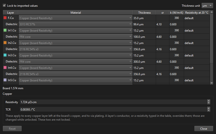
Controls
| Control | What it does |
|---|---|
| Lock to imported values | Ticked (the default), the thicknesses, materials and εr are the ones read from KiCad's board stackup. Untick it to try others: type a new thickness for any copper or dielectric layer, or choose a dielectric's material or type its εr. The layers above and below move with a thickness change, and the total board thickness shows under the table next to KiCad's. Ticking it again goes back to KiCad's values. |
| Thickness unit | Shows and takes the thicknesses in µm,
mm, mil or oz (1 oz = 35 µm). Ounces are a copper weight, so in oz the dielectrics show
in mil. In a µm or mm field a value can also carry its own unit, like 35um
or 0.2mm. KiPI remembers the unit. |
| Material (dielectrics) | Each dielectric's material, from the list KiPI knows: FR4 core and prepreg, polyimide, Kapton, Rogers RO4350B, RO4003C, RO3003 and RT/duroid, PTFE, polyolefin, alumina and aluminum nitride ceramics, and an aluminum metal core. KiCad's own name for the material is listed too when it is not one of these. Choosing a material sets its typical εr (a datasheet value near 1 GHz; type another if your laminate's differs) and its in-plane thermal conductivity k, which the electro-thermal solve uses. Type over k, unlocked, if your laminate's differs; choosing a material again goes back to its typical value. A ⚠ beside k means KiPI did not recognize KiCad's name and took the layer as FR4. Setups from before 0.8.0 with a Thermal tab Laminate k open with that value as every dielectric's k. |
| Material (copper layers) | What each copper layer is
made of. Copper (board Resistivity) uses the Resistivity and TCR below.
Or choose annealed copper, electrodeposited or rolled-annealed copper foil (IPC-4562's
maximum resistivity), silver, gold, aluminum, nickel or tin: this sets the layer's
resistivity, its TCR for the electro-thermal solve, and its thermal conductivity
k for heat spreading. A resistivity typed in the table afterwards wins; setting it
back to default returns the layer to the board's copper. A layer given a
resistivity by hand in an earlier version shows as Custom resistivity. Like the
thicknesses, a layer's conductor is changed only with Lock to imported values
unticked; ticking it again keeps the conductor chosen. |
| εr | Each dielectric's constant, for the AC solve.
default means the stackup gives none (or the material is a metal), and the AC
setup's Default εr applies. |
| Resistivity at 20 °C (table) | A copper layer's own
resistivity, set by its conductor or typed in while unlocked; default uses
the Resistivity below. |
| Resistivity, TCR | Resistivity at 20 °C (annealed copper, 1.724 µΩ·cm, by default) of every layer left at the board's copper and of via plating, and its temperature coefficient (0.00393 /°C for copper), used by the electro-thermal solve. These are setup settings, so they can be changed while the stackup is locked. |
| Reset | Back to KiCad's thicknesses, materials and εr, still unlocked. |
- The stackup and resistivities are saved with the PI setup. An edited stackup is used again the next time the board is opened (unlocked). If a layer has been added, removed or renamed in KiCad since, the log says so and KiCad's stackup is used.
- To compare stackups, solve, edit, and solve again. A stackup change clears the DC results, which were for the old stackup; the AC results stay until a rail is solved again. Reports note a stackup edited in KiPI.
- KiCad's API cannot change a board's stackup yet, so edits stay in KiPI. To keep a stackup you settle on, enter it in KiCad's Board Setup → Board Stackup → Physical Stackup.
- A board snapshot (Save snapshot) keeps KiCad's stackup; the edits live in the setup.
Board panel
The left-hand dock. Its four parts are separated by splitters you can drag.
Nets
Every net on the board. Tick the nets you want to analyze. Ticked nets are drawn in 3D and are the only nets offered in the setup's pin pickers, so a net you need for a VRM, load, series link, capacitor or probe must be ticked first.
| Control | What it does |
|---|---|
| Filter box | Shows only nets whose name contains the text. |
| Power & ground only | Hides signal nets that are not
ticked. Power nets are shown in orange with [PWR], grounds in blue with
[GND]. KiPI recognizes them by name (+3V3, VCC,
GND…), net class, or a zone with several pads. |
| All power | Ticks every power and ground net, keeping any others already ticked. |
| None | Unticks everything. |
The ticked nets are saved with the setup. A board with no saved choice starts with a guess: its largest power planes and the main ground. Building the 3D copper of a big net takes a moment; nets appear as they finish, and Cancel stops the build.
Copper layers
Each copper layer with its thickness and height in the stackup. Untick a layer to hide it; All and None show or hide every layer at once. Hiding layers does not change the result colors; set the color scale to look closer.
Display
| Control | What it does |
|---|---|
| Color | Colors the plain copper by layer or by net. By layer, each layer has its color from the PCB editor's color theme (Preferences → Colors in KiCad), read again on every Load from KiCad; the log names the theme. If the theme cannot be read, KiCad's default theme colors are used. |
| Z scale | Stretches the stackup vertically (1× to 100×) so the layers can be told apart. It only changes the drawing. |
| Opacity | How solid the copper layers and pads are drawn, from 5% to 100%, in both the plain and the result views. Lower it to see the layers beneath; vias stay solid. |
| Vias / Pads / Board | Show or hide via barrels, pads and the board body. |
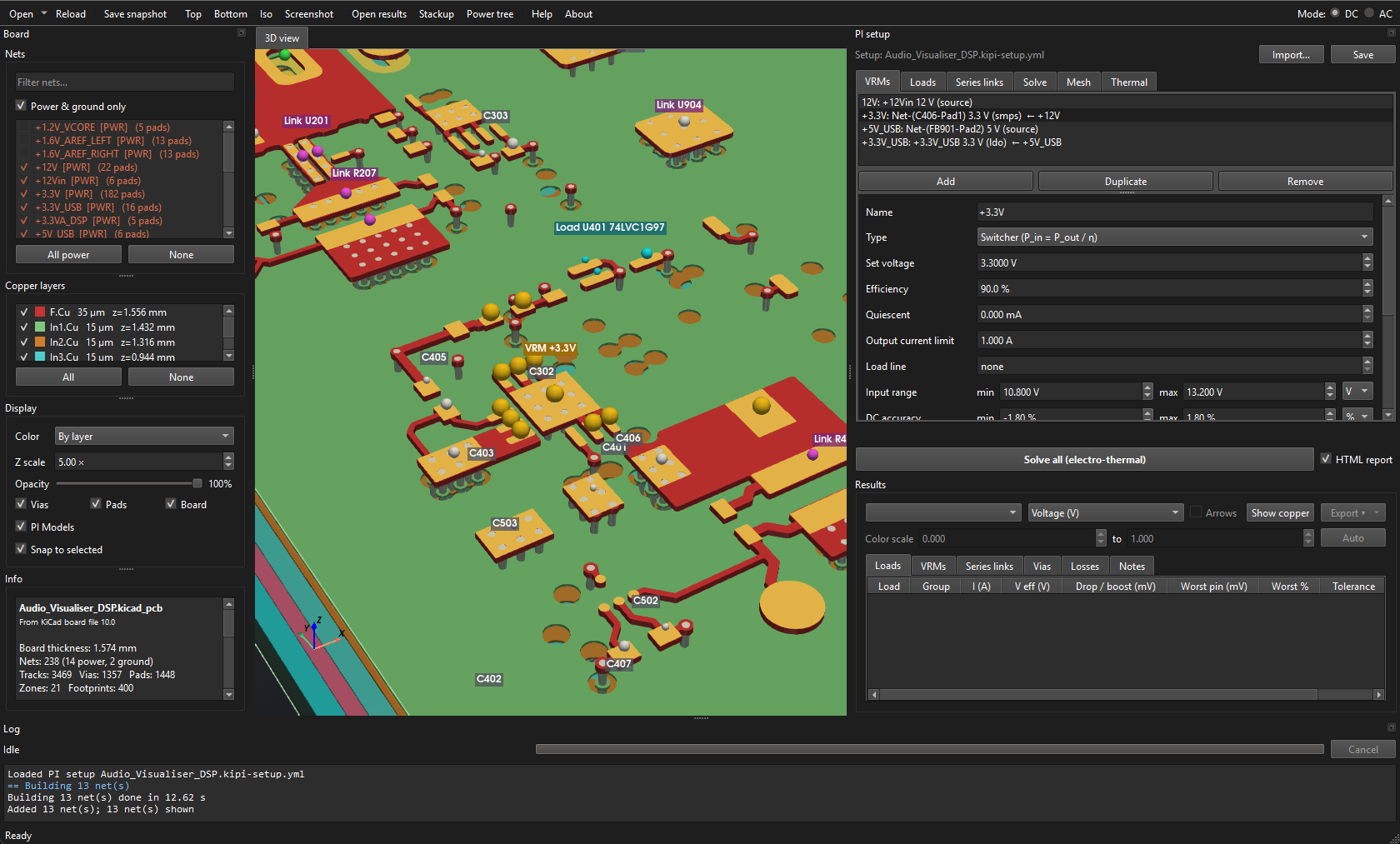
| PI Models | Marks the parts the current
analysis uses on the copper: a dot on each of their pads, larger on the rail's pins and
smaller on ground, with the part's name above. In DC mode those are the setup's
VRMs (green), loads (cyan), series links (magenta) and
capacitors with a model (white). In AC mode the probes (violet) take the
loads' place — the impedance is looked into at a probe, and a load's current says
nothing about it — beside the same VRMs, series links and capacitors. Only pads on a
net shown are marked, and the marks follow setup edits. They are drawn over the plain
copper only, not over results. Unticked to start with. Clicking a VRM, load, series link or probe in the setup's lists marks it in amber, and with Snap to selected ticked brings the view to it; PI Models is left as you set it. Clicking a part's name (or one of its dots) in 3D selects it in the current mode's setup, ready to edit. Either way, the newly selected part blinks red and amber for a few seconds. Capacitors are marked but not selected this way: a model names several parts. |
| Snap to selected | Brings the view to a part when it is picked in the setup's lists (ticked to start with). Available only while PI Models is ticked, since it goes to the part's marks. Untick it to keep the view where it is; the part is still marked and blinks. KiPI remembers the choice. |
| 3D Models | Shows the KiCad 3D models of every part on the board. In the geometry view they are on to start with; over results they start hidden, and ticking 3D Models there shows them too. Each view remembers its own setting. See Part 3D models below. |
Part 3D models
- KiPI asks KiCad's command-line tool,
kicad-cli, to export just the parts it needs, so KiCad finds the model files the same way its own 3D viewer does (STEP and VRML). It runs in the background, the first time the models are shown; each part is read once per board. kicad-clireads the saved.kicad_pcbfile. A part moved since the last save is drawn where it was saved; save the board and click Load from KiCad to update it.- The Z scale stretches the board but not the parts: top-side parts sit on the stretched board at their true height, and on a board made thicker or thinner in the Stackup window.
- Clicks go through the models to the copper beneath, so probing works as without them.
- A part whose model KiCad cannot find is named in the log with the missing path. If
kicad-clior the board file cannot be found, the log says so once and no models are drawn; see Troubleshooting.
Info and Select in KiCad
Shows a summary of the board when it loads, and afterwards whatever you last clicked in 3D: the layer and coordinates, the pad or via hit (net, drill, layer span), and, when results are shown, the voltage, drop, current density, power density and via current at that point. In AC mode it shows the impedance plot's cursor values.
The summary says where the board came from (for example From KiCad PCB editor 10.0.7, and the snapshot file it was opened from). Under Placeholders it lists anything KiPI had to fill in because the source did not give it, such as a default stackup when the board's own is incomplete. Results that depend on a placeholder are only as good as the placeholder.
Select in KiCad selects the picked pad or via in the PCB editor, so you can find it in your layout. It needs a live KiCad connection (not a snapshot), so the plugin has it and standalone KiPI does not.
3D view and mouse
Navigating and probing
| Action | Mouse |
|---|---|
| Rotate | Left-drag |
| Pan | Shift + left-drag, or middle-drag |
| Zoom | Scroll wheel |
| Probe / identify | Left-click copper or a via. The result goes to the Info box and the status bar. Clicks pass through part models. |
In AC mode two more tabs appear beside 3D view: Impedance, with the impedance plot, and Board map, with the mesh and parts of the solve.
Log and progress
The Log dock
The bottom dock shows the current stage, a progress bar, and Cancel, which stops the running task (loading, building nets or solving). The log streams every stage with its timing, solver residuals and warnings: warnings are amber, errors red, stage headers blue.
Each session also writes a log file to kipi/ in your temporary folder
(%TEMP% on Windows, $TMPDIR on macOS, /tmp on Linux).
See Troubleshooting.
DC concepts
Net groups, the power tree and voltage references
Net groups
KiPI solves copper one net group at a time. A group is a net plus every net joined
to it by a series link. For example, +3V3 and
+3V3_FILT joined by a ferrite bead are one group. Each group may be driven by at
most one VRM. Ground nets used by VRM or load ground pins are their own groups.
The power tree
A VRM's input pins make it a load on its upstream net. KiPI solves the tree from the leaves back to the source: downstream rails first, then each VRM's input current (from its output current, efficiency or quiescent current) is applied as a load upstream. So the 12 V input rail carries the current of everything it feeds.
Voltage reference
Voltages are measured against the source's ground (0 V). If ground pins are given, the ground return is solved too and a load's ground rises above 0 V. The figure to compare with the set point is the load's effective voltage: supply minus ground at the load.
Drop and boost
A drop is a pin below the VRM's set voltage. A boost is a pin above it, which happens with remote sense: the VRM raises its output to hold a sense point further down the copper, so pins nearer the VRM sit above the set point. A load is judged by its worst pin, whichever direction.
The pin picker used everywhere pins are chosen
Every "pins" field is three boxes:
- Net: one of the nets ticked in the Board panel. Type to search.
- Part: the parts with pads on that net, busiest first, shown as reference, value and
pad count, e.g.
U4 TPS62130 (3). Type to search (u4is enough). - Pins: optional pin numbers, comma-separated, e.g.
1,2,5. Blank means every pin of that part on that net; the placeholder lists them.
Optional pickers have (none) as their first net.
Pre-filled fields guesses from the board, always yours to change
As you pick pins, KiPI fills in the fields that usually follow from them. Each guess only fills a field you have not set yourself (an empty field, or one it filled in for the previous part), and when the board does not give an answer the field is left as it was. Change anything it fills in: your value is kept.
| When you… | KiPI fills in |
|---|---|
| pick a VRM's output net | Set voltage from the
net's name: +3V3, 3.3V, V1P8, VDD_0V75,
+12V, -5V, VBUS (5 V). A name with no voltage in it
(VCORE, VIN) leaves the voltage alone. |
| pick a VRM's output pins | Ground pins: the same part's pins on its ground net. For an LDO or switcher, Input pins: the same part's pins on its other rail, if it has exactly one. The VRM's Name follows the part while it is still the part's reference. |
| add phases to a VRM | Each new phase repeats the last
one on the parts the next phase likely uses, with the same pin numbers:
|
| pick a load's supply pins | Ground pins: the same part's pins on its ground net. |
| pick a series link's side A | Side B: when the part has pads on just two nets (a resistor, ferrite, fuse, inductor), its pins on the other net. Not for capacitors, or when the other net is a ground. When both sides are on one resistor, Resistance is read from its value. |
| pick a probe's supply pins (AC) | Ground pins: the same part's pins on the probe's ground net, or on its own ground net. |
| Add a VRM, load or series link | The same guesses for its first part. A new series link starts on a two-terminal part between the first two ticked nets that are not grounds. |
How the ground net is found. Ground nets are not always called GND, so KiPI tries, in
order: ground nets the setup already uses (any VRM, load or probe ground pins), nets named like a
ground (GND, PGND, AGND, VSS,
EARTH…), then the board's biggest net (the one with the most pads) if it is not
named like a rail. Only nets ticked in the Board panel are used, except grounds the setup
already uses. Once one VRM or load has ground pins on an unusually named ground, every later
guess uses it.
DC setup tabs
The PI setup dock on the right. Save at its top writes the setup next to the
board (DC and AC share one file). Import… beside it fills the VRMs, loads and series
links from a Tomachie power-tree file (.pdn.json), keeping the settings, thermal
and AC setup. Where the file gives a minimum, typical and maximum, the typical current or
resistance is used, and the log lists what was left out or could not be placed on the
board. Problems that stop a solve are listed in red under the tabs
as you edit. The VRMs, Loads and Series links tabs share one layout: a list with Add,
Duplicate and Remove, and an editor for the selected entry below it.
VRMs tab regulators and supplies
| Field | Meaning |
|---|---|
| Name | Used in the results tables. |
| Type | Source: an ideal supply with no input (connector, bench supply, battery). LDO: Iin = Iout + Iq. Switcher: Pin = Pout / efficiency. |
| Set voltage | The voltage it holds at its output (or sense) pins. Read from the net name when you pick the output net (see pre-filled fields). |
| Efficiency | Switcher only. |
| Quiescent | LDO and switcher: extra input current. |
| Output current limit | Optional. The VRM row shows PASS if its total output current (all phases) is at most this. |
| Load line | Optional, DC only (adaptive voltage positioning). The VRM regulates to its set voltage less this resistance times its output current: what its connected loads and the VRMs it feeds actually draw, so a disconnected load adds no droop. Drops are still measured from the set voltage, so the droop counts against each load's tolerance. The Notes tab, the HTML report and the VRM CSV show the droop and the voltage it regulates to (V target). none holds the set voltage. |
| Dropout | LDO only: the least input-to-output difference at which it still regulates. |
| Input range | Optional input range, min and max on one row, in V or in % from the input rail's nominal voltage (the set voltage of the VRM driving it; e.g. min -10 %, max +10 %). Switching the unit converts the values when that VRM is known. A range in % with no VRM driving the input is a setup error. A VRM whose solved input is outside its range (or an LDO below its dropout) cannot hold its output, and every load it feeds, directly or downstream, is marked VRM OUT OF REGULATION. |
| DC accuracy | LDO and switcher only; used by the AC target calculator. The output's DC error from the datasheet (reference and feedback tolerance, line and load regulation): min and max on one row, in % of the set voltage (e.g. -1 %, +1 %) or in V, the lowest and highest output voltage. |
| Control loop bandwidth | AC only. The AC solve leaves the VRM out of circuit, so it gives the open-loop PDN impedance; below this frequency the converter's loop holds the rail. Probe targets are drawn and judged only above it (see Targets and the VRM bandwidth); none judges the whole target. |
| Phases / Edit phase | Multi-phase regulators. See the multi-phase workflow. |
| Output pins | Where it drives the rail: the output pin, or for a switcher usually the inductor's output side. |
| Input pins | LDO and switcher: where it draws its input. This links it into the power tree. Filled in from the output part when it has one other rail. |
| Ground pins | Optional: solve the ground return as well. Filled in with the output part's ground pins. |
| Sense pins | Optional remote sense (positive). |
| Ground sense pins | Optional negative remote sense on the ground net (needs ground pins). |
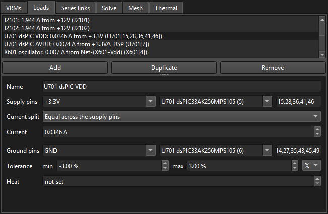
Loads tab parts that draw current
| Field | Meaning |
|---|---|
| Name | Defaults to the supply part's reference. |
| Supply pins | Where the current is drawn. |
| Current split | Equal across the supply pins, or Per pin group: a table of groups, each with its own pins and current. Add pin group adds a row; One group per pin replaces the table with one row per supply pin, sharing the total. ✕ removes a row. Use groups when a part draws different currents on different pins. |
| Current | The load's total current (equal split). Negative values are allowed for parts that source current. |
| Ground pins | Optional: include the load's ground return. Filled in with the supply part's ground pins. |
| Tolerance | Optional min and max on one row, in % from the VRM set voltage (e.g. min -3 %, max +5 %) or in V (e.g. 3.135 to 3.465 V). Either may be left "not set". PASS if every supply pin is within it. Switching the unit converts the values when a VRM drives the load's rail. |
| Heat | Optional, W: the heat the part puts into the board in the electro-thermal solve, when load power is included. Not set: the power it draws. Set it for a part that passes most of its power on, such as a load switch. |
Series links tab parts between two nets
Sense resistors, ferrite beads, fuses, load switches, 0 Ω links: any part that passes DC
from one net to another. Give the part's Side A pins and Side B pins and its
Resistance (DCR); 0 is a short. Picking side A on a two-terminal part fills in side B
on its other net, and when both sides are on the same resistor, the resistance is read from its
value field (10m, 4k7, 0R1, 5 mΩ…).
ESL is used by AC only. A new link starts on a part that bridges the first two ticked
nets that are not grounds, if there is one.
The nets a link joins are solved together as one group, so a group can only hold one VRM. A load pin with no copper path to its VRM is reported, not guessed at (see Loads not connected by copper).
Solve tab choose which net groups to solve
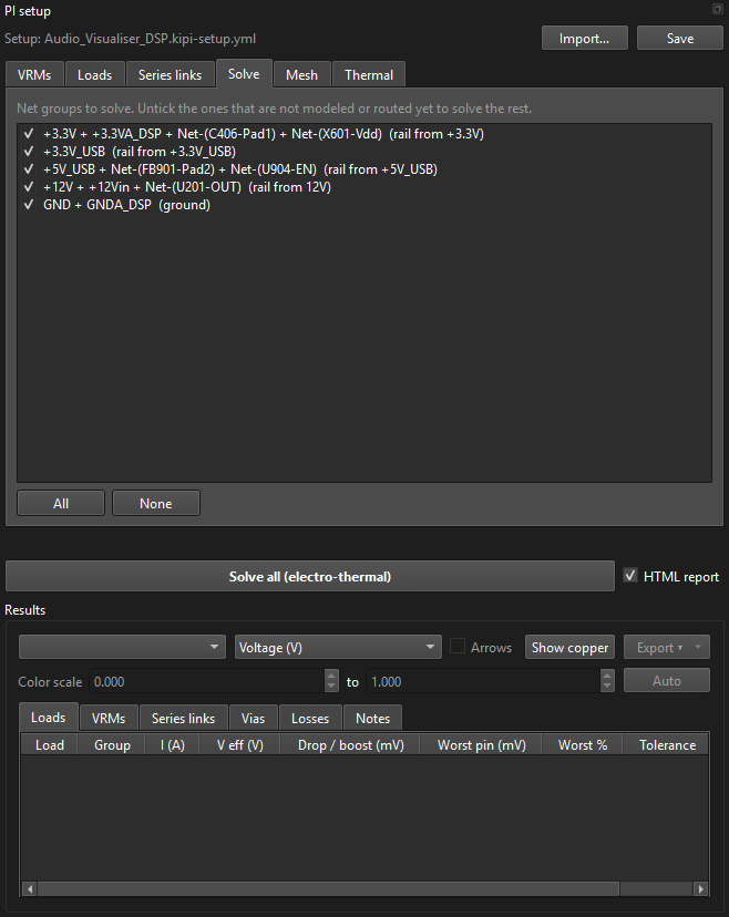
Lists every net group with its role (rail from a VRM, ground, or not driven). Untick groups that are not modeled or routed yet; All and None tick or untick them all. Only ticked groups are validated and solved, and the choice is saved. Where a solved group meets an excluded one:
- A VRM whose output is excluded becomes a constant load on its input pins, drawing the input current its rail would need at nominal voltages.
- A VRM whose input is excluded is treated as an ideal source.
- Ground pins on an excluded ground are ignored.
The Notes results tab lists what was left out and substituted. The Solve button shows how many groups will be solved, e.g. Solve 3 of 5 net groups.
Mesh tab
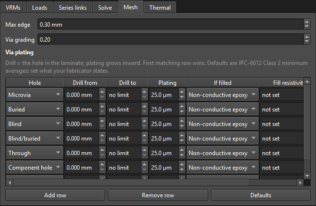
| Field | Meaning |
|---|---|
| Max edge | Largest triangle edge, mm. Smaller is more accurate and slower. Raise it for quick looks at big boards. |
| Via grading | How fast elements grow away from plated holes, where current crowds. Lower keeps the mesh fine further out; 0 turns grading off. |
| Via plating | A table of rules, first match wins: hole type, drill range, plating (µm, growing inward from the drill) and what a filled hole is filled with. A via the KiCad board marks as filled carries its core too when the fill conducts. Defaults: IPC-6012 Class 2 minimum averages. |
The defaults suit most boards; set the via plating your fabricator states.
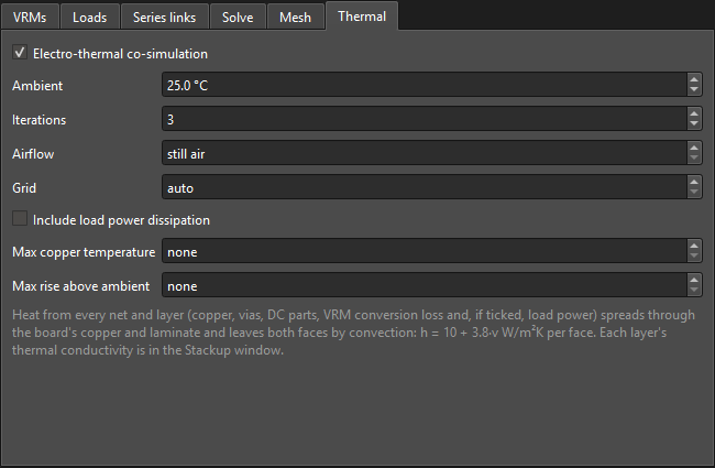
Thermal tab electro-thermal co-simulation, off by default
Tick Electro-thermal co-simulation to let copper losses heat the board, with warmer copper becoming more resistive. KiPI alternates electrical and thermal solves.
| Field | Meaning |
|---|---|
| Ambient | Air temperature around the board. |
| Iterations | Electrical/thermal passes. Three is usually enough; the Thermal results tab shows how much each changed. |
| Airflow | Air speed over both faces, m/s; 0 is still air. The air always flows parallel to the board, along both faces, and its direction is fixed: every point is cooled equally, as if the air stayed at ambient across the whole board, so upstream parts do not warm the air that reaches downstream ones. Convection is h = 10 + 3.8·v W/m²K per face. |
| Grid | Thermal cell size; auto is about 250 cells across the board. |
| Include load power dissipation | Off by default. When ticked, each load heats the board with the power it draws: the sum over its supply and ground pins of pin current × pin voltage, spread over those pins. A load without ground pins is taken as returning at 0 V. |
| Max copper temperature | Optional limit: copper hotter than this on any layer is FAIL. |
| Max rise above ambient | Optional limit on the temperature rise. |
Heat comes from every solved net and layer, vias, DC connections (I²R, at their pins), VRM conversion loss and, with Include load power dissipation, the loads. The report's Component power dissipation table lists the DC connections' and loads' heat. The limits grade the last solve straight away when you change them.
Solving
Solve all, HTML report and Cancel
Solve all saves the setup, meshes every ticked net group and solves the power tree. It is disabled while there are problems (listed in red). If you click it while the 3D view is still building nets, the solve is queued and starts as soon as that finishes.
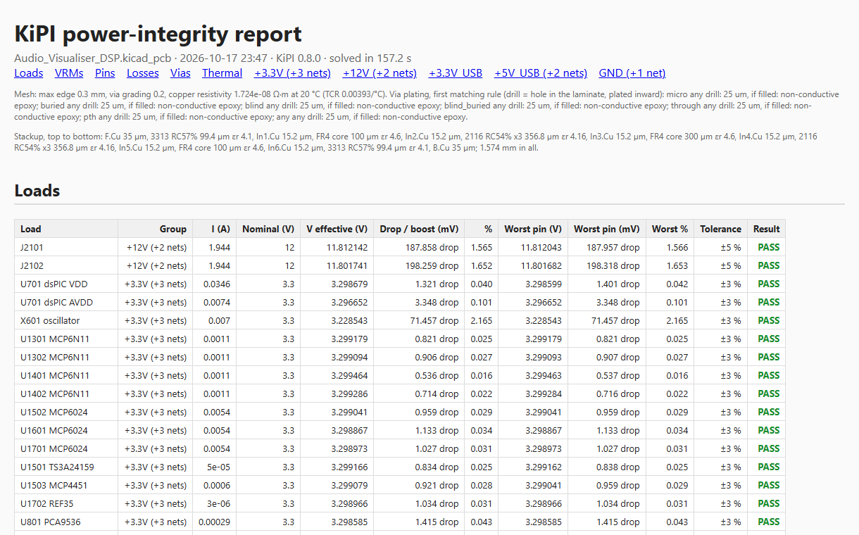
Tick HTML report before solving to also write
<board>_kipi_report_<date>_<time>.html next to the board; the
time stamp keeps each solve's report instead of overwriting the last one. It opens in your web browser when the solve finishes, and
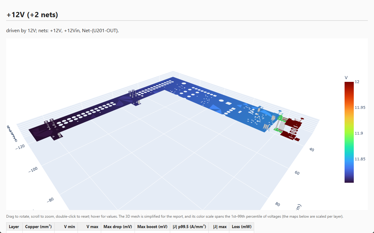
Report opens it again later. The report is a single offline file with every
table, an interactive 3D view of each net group, per-layer statistics and maps, and the
temperature map.
The report's Pins section, and _pins.csv in Export ▾ Tables as
CSV…, list every pin each group was solved with. That covers VRM output, phase, input
and sense pins, load supply and ground pins, and DC connection pins. Each row gives the pin's
position, voltage, drop or boost from the VRM set point (0 V for a ground), and current.
The current is what the pin draws from the copper, so it is negative where current is
delivered into the copper, as at a VRM output. VRM output pin currents are solved, so they
show how the current shares between the pins. A load's current is split equally across its
pins, as the solver applies it, and a DC connection's current across the pins on each
side.
A solve that fails on a setup problem (e.g. no copper path) shows Cannot solve in the Notes tab with the reason. Untick the group with the problem in the Solve tab to solve the rest.
DC results
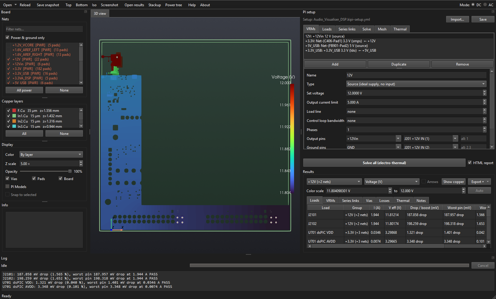
The Results box under the Solve button. Pick a net group and a field to color the copper in 3D.
3D result fields
| Field | Shows | Look for |
|---|---|---|
| Voltage (V) | Copper potential. | The gradient from VRM to load; where the drop happens. |
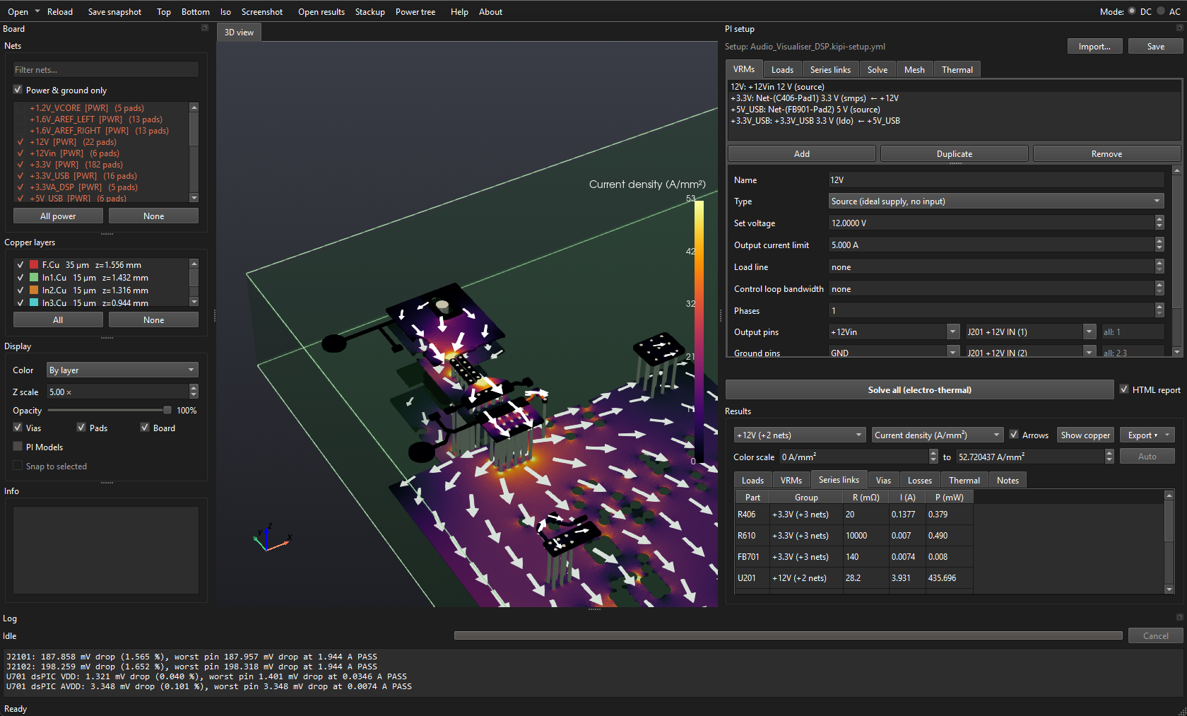
| Current density (A/mm²) | How hard the copper is worked. Tick Arrows to see where and which way current flows: flat white arrows drawn on each layer's copper, top and bottom faces, longer where the current is denser. | Necks, thermal reliefs, narrow traces, plane slots. Clipped at the 99.5th percentile (pad corners spike). |
| Power density (mW/mm²) | Copper loss per area. | Hot spots that the thermal solve will pick up. |
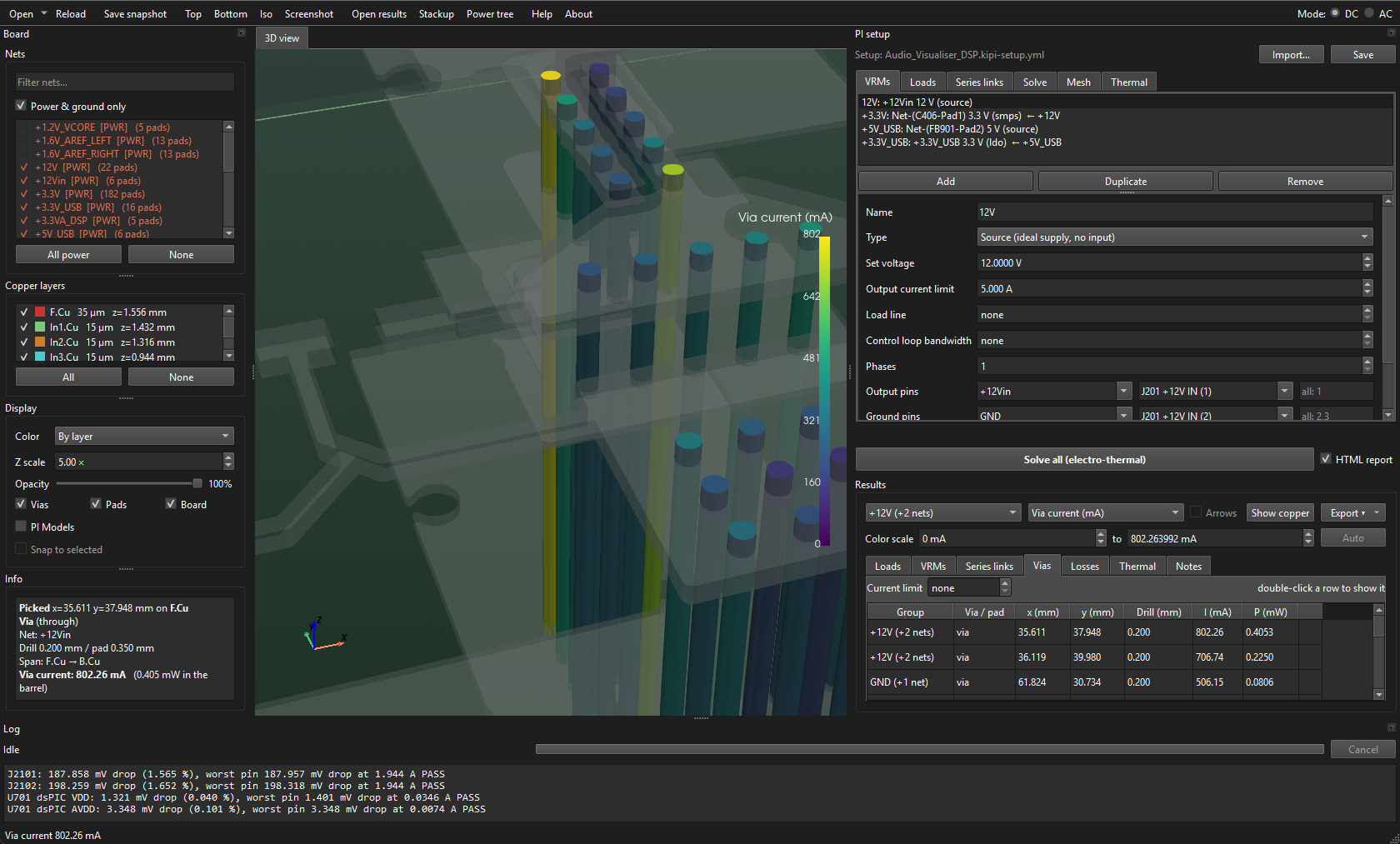
| Via current (mA) | Current in each via barrel. | Vias doing all the work while neighbors idle. |
| Temperature (°C) | Board temperature (electro-thermal only). | Peak location and rise. |
Show copper returns to the plain geometry; pick a group or field again to bring the results back. Click anywhere to probe: Info shows the exact value at that point (not clipped).
Color scale: the minimum and maximum of the colors, under the group and field. Each result starts on its whole range, over every layer whether shown or not. Type limits (or step them with the arrows) to stretch the colors over the part you care about; values outside take the end colors. Limits are kept for each net group and field until Auto fits the whole range again; temperature limits apply to every group, so an ambient-to-limit scale stays put while you switch groups. On the logarithmic power-density scale, a minimum of zero or below falls back to four decades below the maximum.
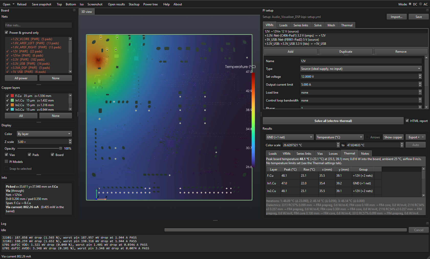
Results tables click a header to sort; again to reverse
| Tab | Columns and use |
|---|---|
| Loads | Current, effective voltage (supply − ground), average drop/boost, worst pin, worst %, tolerance and verdict. Double-click a row to show its group. |
| VRMs | V/I out, V/I in, input power, conversion loss, current limit and PASS/FAIL; a gray row per phase under multi-phase VRMs. |
| Series links | Resistance, current and power in each part. |
| Vias | Every via and PTH barrel, highest current first. The Current limit for PASS/FAIL starts at 1 A, a placeholder; set your own, or 0 for none. Double-click a row to fly the camera to it. |
| Losses | Copper loss per group and layer, in vias and series parts, with the total and each VRM's conversion loss at the bottom. |
| Thermal | After an electro-thermal solve: the hottest copper on each layer, its rise and location, PASS/FAIL against the limits, the iteration history and the dielectric conductivities used. Double-click a row to show its group's temperature. |
| Notes | Solve time, the nets in each group, pin group results, warnings and excluded groups. |
Load verdicts
| Verdict | Meaning |
|---|---|
| PASS | Every supply pin within the tolerance. |
| FAIL | At least one pin outside the tolerance. |
| VRM OUT OF REGULATION | A VRM feeding it, directly or upstream, is outside its input range or below its dropout. |
| NOT CONVERGED | Its group's solve did not converge; the numbers cannot be trusted. See Troubleshooting. |
| DISCONNECTED | None of its supply pins, or none of its ground pins, has a copper or series-link path to its VRM, so its current was left out of the solve. The Notes tab names the pins. See Loads not connected by copper. |
| (blank) | No tolerance set. |
Reading the numbers
- Effective voltage is what the load actually sees: its supply pins minus its ground pins. Compare it with the set point, not the raw plane voltage.
- A supply plane reading above its set point is normal with remote sense or when ground return is solved; see drop and boost.
- Worst pin is the one furthest from the set point; with many pins, one far pin can fail a load whose average looks fine.
- The color scale covers the whole result; type a minimum and maximum under it to look closer.
- Losses are I²R in the copper; VRM conversion loss is the difference between input and output power.
Export and HTML report
| Export ▾ item | Writes |
|---|---|
| Tables as CSV… | One CSV per results table into a folder, plus
<name>_pins.csv: every pin each group was solved with, and its voltage and
current. |
| 3D results for ParaView (.vtm)… | The result meshes, for ParaView or other VTK tools. |
| Save results… | A .kipi-dc-results file, or
.kipi-dc-thermal-results after an electro-thermal solve, that Open
results… reloads without solving, named with the board and the time by default. It holds
JSON and NumPy arrays in a zip, which open on any computer and cannot run code, so it is safe
to share; the 3D views are rebuilt when it opens. |
AC concepts
What the AC analysis models
The AC analysis computes the PDN impedance seen from a probe, a device's supply and ground pins, looking out into the board over a range of frequencies. A device that draws a changing current I from a PDN of impedance Z sees its supply move by about I·|Z|, so keeping |Z| below a target impedance keeps the supply ripple within tolerance.
A solve covers one rail (the nets its VRM drives, plus nets joined to them by series links) against one ground net. It includes:
- The copper, field-solved: plane and trace resistance (with skin effect), the spreading inductance of planes, the capacitance between facing rail and ground copper, cavity resonances, and the inductance of vias and their mounting.
- Capacitors between the rail and ground, each as a series R-L-C from its model. Only the part's own ESL is entered; its mounting (pads, vias, planes) is simulated.
- Series links as their resistance plus ESL.
Capacitors that sit between the rail and ground but have no model are left out, and the results notes list them.
AC setup tabs
Switch Mode to AC. The setup dock becomes the AC setup; it edits the same setup file as DC.
VRMs and Series links tabs shared with DC
The same VRMs and series links as the DC setup; edits in one mode show in the other. Every VRM field can be edited in either mode; the tooltip of a field only DC uses says so. In AC:
- A VRM's output net (and ground pins) define a rail and its default ground for the Rail picker.
- A series link adds its ESL to its resistance. A link leading off the rail to a net that is not part of the solve is left out, with a note. A 0 Ω link with no ESL merges the two nets.
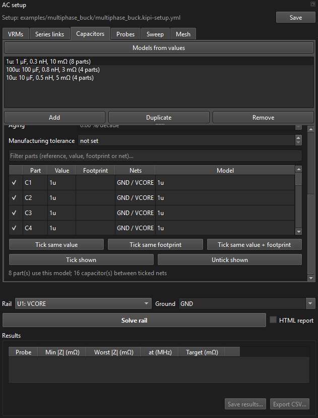
Capacitors tab RLC models and which parts use them
A model is a capacitance, ESL and ESR shared by a group of identical parts. All three are required.
| Control | What it does |
|---|---|
| Models from values | Creates one model per distinct value
among the capacitors that have none yet, named after the value, with the capacitance read
from it, and the voltage rating when the value gives one (10uF 6.3V X5R).
Enter ESL and ESR yourself. |
| Capacitance | Per part, with no DC bias. For a ceramic, enter its Voltage rating to estimate DC bias, or enter the effective value at the rail's voltage if the datasheet gives it. |
| ESL | The part's own inductance (datasheet), not including mounting. |
| ESR | Per part. |
| Voltage rating | The part's rated DC voltage. Class II ceramics (X5R, X7R, X6S…) lose capacitance with DC voltage; with a rating, each part's capacitance is derated by the DC voltage across it: what the last DC solve found across its pads, or else the rail's VRM set point. The Results notes and the HTML report give the voltages and the capacitance left. Models from values fills it in for values naming a class II dielectric. Leave it not set for polymer and electrolytic parts; a model with a C0G dielectric is never derated. |
| Dielectric | The ceramic dielectric (C0G, X7R, X5R, Y5V…), for
aging and temperature. Picking one fills in its typical aging rate, and with a
Temperature in the Sweep tab the capacitance follows the dielectric's typical
curve from its rated value at 25 °C (X7R: −4 % at 85 °C and −12 % at 125 °C; Y5V: −75 %
at 85 °C; C0G: flat). Leave it unset for polymer and
electrolytic parts, which are then not aged. Models from values reads it from the
value (NP0 counts as C0G). |
| Aging | Capacitance lost per decade of hours operated, in % (X7R about 2, X5R about 3, Y5V about 7; C0G does not age). Enter the datasheet's rate if it gives one. Used when Capacitor aging is ticked in the Sweep tab. |
| Manufacturing tolerance | Optional: the part's capacitance tolerance, in % of nominal, from its datasheet or its value code (J is ±5 %, K ±10 %, M ±20 %). Used when Capacitor manufacturing tolerance is ticked in the Sweep tab, which solves the model at the low end of it. Leave it not set for a part whose entered capacitance is already the figure you want simulated. |
| Kept at rating | How much of its capacitance the part keeps at its rated voltage, from the datasheet's DC bias curve (40 % by default; often 30 to 50 %, and less for smaller cases). Between 0 V and beyond the rating, the capacitance follows C / (1 + k (V / Vrated)1.5), a typical X5R/X7R curve's shape. |
| Filter box | Narrows the parts table by reference, value, footprint, net or model. |
| Parts table | Every capacitor (reference C…) whose pads
are all on ticked nets, across two nets, with its footprint (hover for the library).
Tick a part to give it this model; it moves from any other model. Grayed rows already
belong to another model, named in the last column. Click a column header to sort by it. |
| Tick same value / footprint / value + footprint | Ticks every part matching the selected row: the same value, the same library footprint, or both (e.g. only the 0402 100 nF parts, whose ESL differs from the 0603 ones). |
| Tick shown / Untick shown | Applies to every row the filter shows. |
Probes tab where the impedance is measured, and its target
| Field | Meaning |
|---|---|
| Name | Shown in the plot legend and the table; follows the supply part by default. |
| Supply pins | The device's power pins. Picking a part also picks its ground pins if it has any. |
| Ground pins | Must be on the ground net being simulated. |
| Target | Flat, up to a frequency, or Custom (piecewise linear). |
| Target |Z| / Target frequency | Flat target: PASS if |Z| stays at or below it from the VRM's control loop bandwidth up to the frequency (none: to the end of the sweep). |
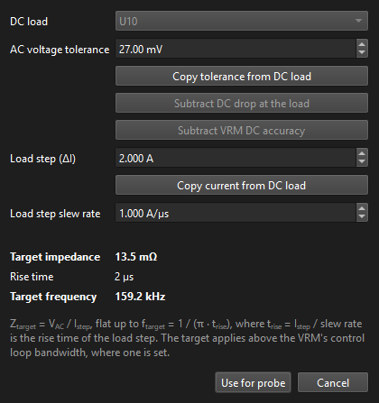
| Calculator… | Opens the Target Impedance/Frequency Calculator. |
| Custom points | Frequency/|Z| corner points, joined by straight lines on the log-log plot. Below the first point the first |Z| holds, above the last the last holds. Add point adds one a decade above the last; ✕ removes one. |
From DC load adds a probe on the same supply and ground pins as a DC load picked from its dropdown. The dropdown also lists the input of every LDO and switcher, one entry per phase (e.g. VR4 phase 2 input): a regulator's input pins load the rail feeding it just as a device does.
A rail can have several probes, e.g. one per device; they are all solved together and each sees the others as open circuits.
Targets and the VRM bandwidth
The AC solve leaves the VRM out of circuit: it gives the open-loop PDN impedance, which keeps rising toward low frequency. In the real circuit the converter's control loop holds the rail below its bandwidth. So when the rail's VRM has a Control loop bandwidth, a probe's target (flat or custom) applies only from that frequency up:
- the plot draws the target only above the bandwidth, and marks the bandwidth with a dotted line;
- PASS/FAIL, the worst |Z| and the margin only look above it. Without a target, the worst |Z| is the highest above the bandwidth;
- the cursor shows "none here" below it.
Fallback: if the bandwidth is at or above a flat target's frequency, or above the whole sweep, no frequencies are left to judge. That probe's target is then judged over its whole range, as if the VRM had no bandwidth, and a note in the results says so.
Target Impedance/Frequency Calculator
Works out a flat target from the device's transient spec:
- DC load: the DC load whose tolerance and current the copy buttons use. A load on the probe's own supply and ground pins is used directly. Otherwise the dropdown offers the loads on the probe's part: supply pins on the same footprint, and ground pins too where the load has them. An LDO's or switcher's input pins count as a load too: its Input range is the tolerance, and its input current and the DC drop at its input pins come from the last DC solve.
- AC voltage tolerance: how far the supply may move during a load transient, e.g. the AC part of a ±3 % spec on a 0.9 V rail: 27 mV.
- Copy tolerance from DC load fills the AC voltage tolerance from a DC load's tolerance: ± its tighter side, from the voltage of the VRM feeding it (2 % for -2 % / +5 %). A DC tolerance is the whole budget, and the DC drop uses up part of it, so lower the value if the AC part is smaller.
- Subtract DC drop at the load takes the DC drop the copper causes at the selected load's own pins off the AC voltage tolerance, so what is left is the budget for the transient. It reads the last DC solve: its effective voltage there (supply pins minus ground pins) against the set voltage of the VRM driving it, so solve the power tree on the DC tab first — without a result for that load the button stays disabled and says so. A load above its set voltage (a remote-sensed VRM raises pins near it) has its boost subtracted just the same, since it eats the same symmetric window. Each click subtracts again.
- Subtract VRM DC accuracy takes the DC accuracy of the LDO or switcher driving the probe's rail off the AC voltage tolerance: the larger side of it (20 mV for -1 % / +2 % of 1 V), as the output may already sit that far from its set voltage. It shows a menu when several VRMs drive the rail; each click subtracts again.
- Load step (ΔI): the size of the current step.
- Copy current from DC load fills the load step from a DC load's current, a step from no load to all of it. Lower it if the device's current steps by less.
- Load step slew rate: how fast it steps, A/µs; 10 A/µs until you change it.
Then Ztarget = VAC / ΔI, flat up to ftarget = 1 / (π · trise), with trise = ΔI / slew rate. Use for probe fills the probe's target fields; the inputs are remembered for next time. The target applies above the VRM's control loop bandwidth (Targets and the VRM bandwidth).
The target impedance method was introduced by L. D. Smith, R. E. Anderson, D. W. Forehand, T. J. Pelc and T. Roy, "Power Distribution System Design Methodology and Capacitor Selection for Modern CMOS Technology," IEEE Transactions on Advanced Packaging, vol. 22, no. 3, pp. 284–291, Aug. 1999.
Sweep tab
| Field | Meaning |
|---|---|
| Start / Stop | Frequency range. |
| Points per decade | Resolution of the plotted curve. Cheap: the parts are evaluated at every point. |
| Field solves per decade | How often the copper itself is solved; in between, its response is interpolated (smoothly, it varies slowly). Every point solves the copper at each sweep frequency: exact and slowest. Raise this if sharp plane resonances look under-resolved. |
| Capacitor DC bias | Ticked (the default), the capacitor models with a Voltage rating are derated by the DC voltage across each part. Untick it to solve with every model's capacitance as entered. |
| Capacitor manufacturing tolerance | Ticked, every capacitor model with a Manufacturing tolerance is solved at the low end of it: the tolerance is subtracted, so a ±10 % model keeps 90 % of its capacitance and a ±20 % model 80 %. That is the worst case for a PDN, where too little capacitance raises the impedance. Models without a tolerance are unchanged. This multiplies with the DC bias estimate, aging and temperature. Off by default. |
| Temperature | Not modeled (the default): copper at 20 °C and capacitors at their rated values. Fixed: the whole board at Board temperature. From DC thermal co-simulation: each copper triangle and capacitor at the temperature the last DC solve with thermal co-simulation found there; DC results opened from a file work too. Without one, the AC solve uses the Board temperature and says so. The copper's resistivity follows its temperature coefficient (from the DC settings), and models with a dielectric follow its temperature curve. |
| Board temperature | The temperature when Fixed, and where the thermal co-simulation gives none. |
| Capacitor aging | Ticked, every capacitor model with a dielectric loses its aging rate for each decade of Hours operated past 1000 hours (the usual reference age of the rated capacitance): an X7R part at 2 %/decade keeps 96 % after 100,000 hours. This multiplies with the DC bias estimate. Off by default. |
| Hours operated | How long the capacitors have aged, in hours (8760 a year; 87,600, ten years, by default). Heating a ceramic past its Curie point, as in reflow soldering, restarts its aging. While aging is ticked, a slider under it sets the hours from 1000 to 1,000,000 on a log scale, with the time in years beside it. |
Mesh tab
| Field | Meaning |
|---|---|
| Max edge | Largest element, mm. |
| Via grading | Element growth per mm away from plated holes. |
| Min edge (at holes) | Element size at plated holes. The mesh here decides the via and mounting inductance. |
| Loss tangent | Dielectric loss (FR4 about 0.02). Damps the plane resonances. |
| Default εr | Dielectric constant where the stackup gives none. Every other dielectric uses the εr from KiCad's board stackup (Board Setup → Physical Stackup); a dielectric made of several sublayers gets their series combination. The log and the HTML report list the εr used for each dielectric. |
Copper resistivity and the via plating rules come from the DC setup's Copper and Mesh tabs.
Solving a rail
Rail, Ground and Solve rail
Below the tabs: Rail lists each VRM and its output net; Ground lists the ticked nets with grounds first, defaulting to the VRM's ground pins' net. Solve rail saves the setup and runs the sweep; problems that stop it are listed in red above. The log shows the field solves as they go.
Tick HTML report next to Solve rail to also write
<board>_<rail>_ac_report_<date>_<time>.html next to the
board after each rail's solve;
the report opens in your web browser when the rail finishes solving, and Report opens
the shown rail's report again later. See AC HTML report.
Each rail keeps its last result: switch Rail to look at another rail's curves without solving again. If you change the rail while a solve is running, the result is kept for its own rail and the notes say so.
AC results
Impedance plot and cursor
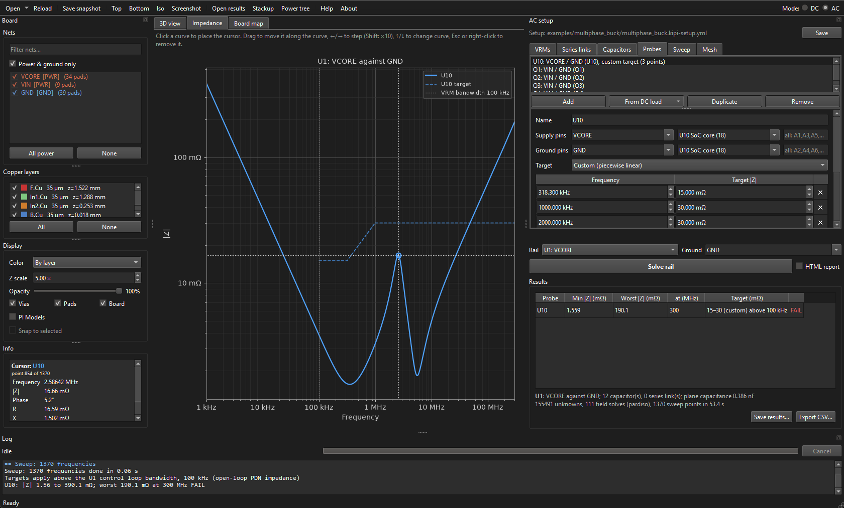
The Impedance tab in the middle plots |Z| against frequency on log-log axes: one solid curve per probe and, dashed in the same color, its target. Hovering shows every probe's |Z| at the frequency under the mouse in the line above the plot.
Cursor
| Action | Input |
|---|---|
| Place on the nearest curve | Left-click |
| Move along the curve | Drag, or ← → (with Shift: 10 points) |
| Switch curve | ↑ ↓ |
| Remove | Esc or right-click |
The Info box shows the cursor's frequency, |Z|, phase, R and X, the reactance as an equivalent L or C, the target there with PASS/FAIL and the margin in dB (positive is below the target), and every other probe's |Z| at the same frequency.
Screenshot… in the toolbar saves the plot as a PNG while its tab is showing.
Board map
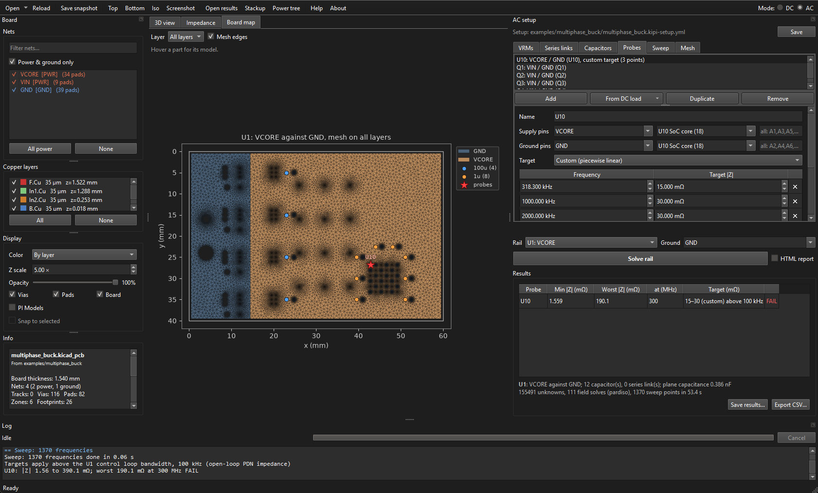
The Board map tab shows the solve from above, as in the HTML report: the solver's mesh of the rail (copper colored) and its ground (blue-gray), the board outline, the probes as red stars, and the capacitors in the model as dots, one color per capacitor model. Capacitors between the rail and ground that have no model, and so are left out, are crossed. The view is fixed, always fitted to the board.
The map fills in while the rail solves: the parts as soon as the solve starts, then the mesh once it is built. The tab comes to the front for the solve; the Impedance tab comes back to the front when the results arrive.
| Control | Does |
|---|---|
| Layer | The copper layer whose mesh is shown, or All layers (the rail drawn over its ground). |
| Mesh edges | Draws the triangles' edges. Untick it to see the copper alone. |
| Hover a part | Its reference, value, side and capacitor model (C, ESL, ESR). |
The map belongs to each rail's result, so switching Rail shows that rail's map, and saved results keep it. Results saved by KiPI before 0.7.2 have no map.
Results table and notes
| Column | Meaning |
|---|---|
| Min |Z| | Lowest impedance in the sweep. |
| Worst |Z| / at | With a target: the point where |Z| comes closest to, or furthest over, the target (within the target's frequency range). Without one: the highest |Z| in the sweep. |
| Target | The flat level, or the custom mask's range. |
| Verdict | PASS if |Z| is at or below the target everywhere it applies. |
Below the table, the notes give the rail's nets and ground, the number of capacitors and
series links included, the total plane capacitance, the solve size and time, capacitors left
out for having no model, and any warnings. Export CSV… writes |Z|, R and X of every probe
at every frequency. Save results… writes every rail solved so far to a
.kipi-ac-results file (named with the board and the time by default);
Open results… in AC mode brings them back, each
under its VRM in Rail. Rails whose VRM is no longer in the setup are left out.
AC HTML report
With HTML report ticked, each rail's solve also writes
<board>_<rail>_ac_report_<date>_<time>.html next to the
board; the time stamp keeps every solve's report. Like the DC report, it is a single offline file you can email. It holds:
- a summary and the probe table: pins, minimum and worst |Z|, the target, the margin in dB at the worst point (positive passes), PASS/FAIL, and an overall verdict;
- an interactive impedance plot of |Z| at every probe, with the targets dashed. Drag to zoom, double-click to reset, hover for f, |Z|, R and X. Click a legend entry to hide or show a curve. The grey dotted curves, hidden at first, are each capacitor model on its own (one part, without mounting), useful for matching dips to capacitor banks;
- a board map seen from the top: the board outline, the rail's copper on every layer merged, the probes as stars and each capacitor colored by its model. Capacitors left out for having no model show as grey crosses;
- the capacitor models (C, ESL, ESR, self-resonance, how many parts and which), the series links, the sweep, mesh and copper settings, and the solver's size, backend and time;
- notes: capacitors left out and any warnings.
If the report can't be written, the log says why; the solve's results are kept either way.
Reading an impedance curve
- Falling at −20 dB/decade (|Z| ∝ 1/f): capacitive. At the low end this is the bulk capacitance; since the VRM is not modeled, the curve keeps rising toward low frequency.
- Dips: series resonances, where a capacitor bank's C and its ESL plus mounting inductance cancel. The depth is set by ESR.
- Peaks between dips: anti-resonances, where one bank's inductance resonates with the next bank's capacitance. These are usually where a target fails. Fix them with more or lower-ESL parts, more value overlap between banks, or extra damping (ESR).
- Rising at +20 dB/decade (|Z| ∝ f): inductive. The capacitors' ESL and their mounting (pad, via and spreading inductance) dominate. Place the cursor here: Info shows it as an equivalent inductance. Shorter, wider connections and more vias lower it.
- Sharp peaks at high frequency: plane-pair cavity resonances. Their frequencies come from the board's dimensions and stackup.
- Phase near −90° is capacitive, near +90° inductive, near 0° resistive.
Step-by-step workflows
1. A first DC IR-drop check of one rail
- Tick the rail and its ground in the Nets list; untick everything else.
- VRMs tab: Add a Source on the regulator's output pins at the set voltage. Add its ground pins.
- Loads tab: Add each consumer with its current, tolerance and ground pins.
- Solve all. Check the Loads table. For a FAIL, double-click the row, choose Voltage, and click around the load's pins to see where the drop comes from.
- Switch to Current density with Arrows to find the bottleneck, change the layout in KiCad, and use Load from KiCad and Solve all again.
2. A full power tree (input → switcher → LDO)
- Tick every rail in the chain and the ground.
- Add the input as a Source (e.g. the 12 V connector).
- Add the switcher as Switcher with its efficiency, output pins (inductor), Input pins on the 12 V net, and ground pins.
- Add the LDO as LDO with its quiescent current, dropout and Input pins on the switcher's output.
- Add loads on each rail and solve. The VRMs table shows each converter's input current, which includes everything downstream, and its conversion loss.
- Set Input range and Dropout to catch a regulator starved by upstream drop: its loads show VRM OUT OF REGULATION.
3. A multi-phase regulator
- Add the VRM and set phase 1's output pins (its inductor), input pins and ground pins.
- Set Phases to the number of phases. Each new phase takes the next parts in
sequence (phase 1 on
L1andQ1gives phase 2L2andQ2), or the same parts on the next sheet of a board annotated by sheet (L101 → L201), or copies the previous phase when there is no next part. - Choose each phase in Edit phase to check its pins, and change any that are wrong.
- Set the shared set voltage, type, efficiency and sense pins once.
Each phase carries an equal share of the output current and settles at whatever voltage its copper needs. The VRM regulates its sense pins or, without them, the average of its phase outputs. The VRMs table lists each phase under its VRM: unequal phase voltages show a layout imbalance.
4. Remote sense
- On the VRM, set Sense pins to the point the feedback trace connects to (often the load's supply pins).
- For differential sensing, also set Ground sense pins on the ground net (the VRM needs ground pins too).
- Solve. The sense point sits exactly at the set voltage; pins nearer the VRM read above it (a boost). The tolerance check catches both directions.
5. Solving only part of the board
When some rails are not routed or modeled yet, open the Solve tab and untick their groups. The rest solves, with the substitutions described under Solve tab. Untick the group a Cannot solve message names to get past a setup problem while you fix it.
6. Thermal and current capacity checks
- Thermal tab: tick Electro-thermal co-simulation, set ambient and airflow, and limits for maximum temperature and rise.
- On the Vias results tab, set the Current limit per via from your fab's via current rating (it starts at 1 A).
- Solve all (electro-thermal). Read the Thermal tab for the hottest point per layer, and sort the Vias tab by current for overloaded vias.
- Use the Temperature field to see the map; double-click a Thermal row to jump to its group.
7. Designing decoupling to a target impedance (AC)
- Make sure the rail has a VRM (Source is fine), and tick the rail, its ground and any nets joined by series links.
- Switch to AC. Capacitors tab: Models from values, then enter ESL and ESR for each model from the datasheets.
- Probes tab: add a probe on the device's power and ground pins. Use the calculator for the target, or a custom mask from the device vendor.
- Solve rail. In the plot, put the cursor on the worst peak (the table's Worst |Z| tells you where).
- Change capacitor models (values, counts by re-assigning parts) or the layout, and solve again. Each probe's margin in dB shows the improvement.
- To compare rails, solve each and switch between them with Rail; each keeps its last result for the session.
Capacitors listed under "have no model and were left out" are not part of the result: give them a model or confirm they really do not belong on this rail.
8. Sharing a board and its results
- Save snapshot… stores the board; anyone with KiPI can open it with Open snapshot…, or with Open… in standalone KiPI, without KiCad or your design files.
- Keep
<board>.kipi-setup.ymlin version control next to the board. - Tick HTML report for a single file you can email: it needs nothing but a browser.
- Export ▾ → Save results… (DC) or Save results… (AC) lets you reopen a long solve later with Open results….
Files KiPI reads and writes
File reference
| File | What it is |
|---|---|
<board>.kipi-setup.yml | The setup: ticked nets, VRMs, loads, series links, mesh, copper and thermal settings, capacitor models, probes and the sweep, in YAML. Saved next to the board on Save and on every solve. |
<board>.kipi-setup.json | A setup saved by KiPI
before 0.8.0. It still opens, with a warning, when there is no .yml setup;
the next save writes the .yml and leaves the JSON file alone. JSON setups
are deprecated: a future KiPI will stop reading them. |
*.kipi.json.gz | A board snapshot (copper, stackup, pads, vias, parts). |
*.kipi-dc-results | A saved DC solve: JSON and NumPy arrays in a zip. |
*.kipi-dc-thermal-results | A saved electro-thermal solve (DC with the board temperature), in the same format. |
*.kipi-results | DC results saved by KiPI 0.7 and earlier, as Python pickles, which can run code; KiPI asks before it opens one, and they are deprecated. |
*.kipi-ac-results | Saved AC results, every rail solved, in the same format. |
<board>_kipi_report_<date>_<time>.html | The DC HTML report. |
<board>_<rail>_ac_report_<date>_<time>.html | An AC rail's HTML report. |
*.csv | DC tables, or an AC rail's impedance. |
*.vtm | DC 3D results for ParaView. |
| KiPI's environment | Standalone only: the packages the launcher
installed, in %LOCALAPPDATA%\KiPI\venv (Windows),
~/Library/Application Support/KiPI/venv (macOS) or
~/.local/share/kipi/venv (Linux), with the launcher's logs in
logs beside it. python kipi_launcher.py --reset deletes
it. |
kipi-<user>.lock,kipi-standalone-<user>.lock |
In the temporary folder while the plugin, or standalone KiPI, is open, so a second one brings the first to the front. It names the owner's process, so one left behind by a crash is ignored. |
<board>.kicad_prl | KiCad's own local project
settings. kicad-cli may create it next to the board the first time it exports
part models, if the project has none yet. |
kipi-<date>-<time>-<pid>.log | The session
log, in kipi/ under the temporary folder, with a matching
.crash.log. The last 15 sessions are kept. |
Troubleshooting
The KiPI button does not appear in KiCad
Enable Preferences → Plugins → Enable KiCad API and restart the PCB editor. The first start builds a Python environment and downloads a few hundred MB, which can take several minutes. If the button never appears, right-click the action in Preferences → Plugins and choose Recreate Plugin Environment. On macOS, select a Python 3.10–3.13 interpreter there.
"KiPI works with one KiCad at a time"
More than one KiCad project manager or standalone PCB editor is open, and
KiPI cannot tell which one holds your board. Close the others (the message lists them with their
process IDs) and start KiPI again from the PCB editor of the board you want. If you know the
check is wrong, set the environment variable KIPI_ALLOW_MULTIPLE_KICAD=1 to skip it.
If the running programs cannot be listed, KiPI carries on.
Standalone KiPI does not set up or start
- No suitable Python: the launcher needs Python 3.10 to 3.13 and names the ones
it found. Install one from python.org (on Linux, also
python3-venv). - The setup failed: the message says why, and the launcher's log (in
logsnext to KiPI's environment) has everything the installer printed. Check the network connection and free disk space, then start the launcher again; it picks up where it stopped.python kipi_launcher.py --repairstarts over. - A message box says to use a terminal: that Python has no tkinter for the setup
window. Run
python kipi_launcher.pyin a terminal and answer there.
A KiCad board file opens with copper missing, or not at all
- Zones have no copper: they were saved unfilled, and KiPI does not fill zones. Fill them in KiCad (B), save, and Reload. The board summary lists unfilled zones under Placeholders.
- Copper looks out of date: KiCad fills zones when asked, not on every edit. Refill and save in KiCad after moving copper.
- "saved by KiCad 6 or older": open the board in KiCad 7 or later, save it, and open it again.
An ODB++ job opens with nets or copper missing
- "not an ODB++ job": the archive has no
matrix/matrixfile, e.g. a zip of Gerbers. Export ODB++ from the design tool. - "no netlist": the job has no
eda/data; export it with its netlist, or KiPI cannot tell which copper is which net. - A net from KiCad has a different name: KiCad's ODB++ export writes spaces in net names as underscores. Pick the net again in the setup.
- A copper drawing carries no current: some exporters (KiCad among them) do not say which net drawn copper is on. KiPI gives it the net of the copper it touches; on its own it has none.
Clicking the KiPI button does not open a new window
KiPI is already open, perhaps minimized or behind KiCad; the button brings it
to the front. If it is not open and still does not start, check the session log for a stale lock
and delete kipi-<user>.lock (kipi-standalone-<user>.lock for
standalone KiPI) from the temporary folder.
No part models are drawn
- Check 3D Models is ticked in Display. Over results it starts unticked.
- The log says why. KiPI needs KiCad's
kicad-cli: it looks in the connected KiCad, the PATH, the usual install folders and a Flatpak KiCad. Otherwise set the environment variableKIPI_KICAD_CLIto its full path. - It also needs the board's
.kicad_pcbon disk, next to the project or the snapshot. A snapshot opened on another machine usually has none. - A part whose model file KiCad cannot find is named in the log with the missing path; KiCad's own 3D viewer shows the same gap. Fix the path in the footprint's 3D model settings and save the board.
A net is missing from the pin pickers
Pickers only offer nets ticked in the Nets list. Tick it (untick Power & ground only or use the filter to find a signal net).
Loads not connected by copper
Before solving, KiPI checks that every load pin has a path to its VRM through copper or series links, and its ground pins to the ground reference. A pin without one draws nothing, and the Notes tab lists it:
- Some pins of a load unconnected: its current is drawn through its other pins. A pin group with no pin connected draws nothing.
- No supply pin, or no ground pin, connected: the load's current is left out of the solve and it shows as DISCONNECTED.
- A rail where no load is connected at all: the solve stops with Cannot solve. So does an unconnected VRM pin.
The cause is usually unrouted copper, an unfilled zone (keep Refill zones on), or a part in series that needs a series link. Show the net in 3D and look for the gap.
The drop is larger than expected
Thermal reliefs, necked traces and too few vias dominate DC drop. Use Current density with Arrows, and the Vias table sorted by current. Compare the 3D copper with KiCad: KiPI only sees filled copper.
NOT CONVERGED
The iterative solver did not reach its tolerance on a very large group. Raise Max edge to shrink the problem, or install the optional PARDISO solver (see the README) for a direct solve of up to 1M unknowns.
Solves are slow
Raise Max edge, analyze fewer nets at once, and untick unneeded groups in the Solve tab. In AC, lower Field solves per decade or raise Min edge. Large planes are cheap; long fine traces are not. PARDISO helps a lot on large boards (Windows and Linux, x86-64).
An AC curve looks wrong
- Check the notes for capacitors left out for having no model.
- Check every model's ESL and ESR units (nH and mΩ).
- Check the probe's ground pins are on the ground being simulated.
- Remember the VRM is not modeled: the low-frequency rise is expected.
- Raise Field solves per decade if resonances look jagged.
Reporting a bug
Open an issue at github.com/drewsum/KiPI/issues.
Attach the session's .log and .crash.log, the text from About → Copy
version info, and if you can, a board snapshot and setup file that show the problem.
Glossary
Terms used in KiPI
| Term | Meaning |
|---|---|
| PI | Power integrity: delivering clean, correct supply voltage. |
| PDN | Power distribution network: regulators, copper, vias and capacitors between a supply and its loads. |
| VRM | Voltage regulator module: any regulator or supply. |
| IR drop | Voltage lost to current flowing through copper resistance. |
| Net group | Nets solved together because series links join them. |
| Remote sense | A VRM regulating the voltage at a point other than its output. |
| PTH | Plated through hole (pads with plated drills). |
| ESR / ESL | Equivalent series resistance / inductance of a part. |
| DCR | DC resistance of a series part. |
| Target impedance | The highest PDN impedance that keeps supply ripple within tolerance for the expected load steps. |
| Anti-resonance | An impedance peak where one capacitor bank's inductance resonates with another's capacitance. |
| TCR | Temperature coefficient of resistance. |
KiPI is free software under the GNU GPL v3 or later. Source and issues: github.com/drewsum/KiPI.